![]()
![]()


Last updated: July 2026
1 Introduction
This manual introduces phonokit and its functions. phonokit is a Typst package designed to streamline the creation of phonological structures while maintaining typographical precision. Typst is a programming language for typesetting — there is a great tutorial here and an introductory YouTube series here.
The package provides intuitive functions for IPA transcription, prosodic representations (syllables, moras, feet, prosodic words, metrical grids), sonority profiles, IPA vowel charts and consonant tables, autosegmental phonology, multi-tier representations, feature geometry, SPE feature matrices, Optimality Theory tableaux, Harmonic Grammar, Noisy Harmonic Grammar, Maximum Entropy grammars, Hasse diagrams, numbered linguistic examples, and helper symbols. The main goals of phonokit are to minimize effort and maximize quality.
The GitHub repository for the package can be found at guilhermegarcia/phonokit. Comments, suggestions and bug reports are welcome — please open an issue in the repository.
1.1 Installation
Typst packages are loaded with the #import function at the top of your typ document. Replace X.X.X with the version you wish to import:
Package import (Typst Universe)
#import "@preview/phonokit:X.X.X": *Alternatively, if you want the most up-to-date version, download or clone the repository and load the package locally:
Local import
#import "phonokit/lib.typ": *You may need a symlink depending on how you structure your files, since Typst restricts imports to files within the compilation root and its subdirectories.
1.2 Font
All functions in phonokit require the Charis font to work as intended out of the box (SIL International 2025). As of version 0.3.7, the user can set a global font to be used by the package throughout the document:
Setting the font
#import "@preview/phonokit:0.5.12": *
#phonokit-init(font: "New Computer Modern")  // add to the top of your document
2 IPA
IPA transcription is likely the most commonly used feature when typesetting documents in phonology. Typst supports unicode input directly, so technically you can type IPA symbols without a dedicated package. However, you may prefer to use a function-based workflow for that, especially if you’re coming from \(\LaTeX\). phonokit accomplishes that with the #ipa() function, which takes a string as input. Crucially, the function uses the familiar tipa input (Rei 1996), with a few exceptions (e.g., secondary stress is represented by a comma ,, not by two double quotes "").
2.1 Transcription
Symbols introduced by two backslashes \\ must not have adjacent characters. For archiphonemes, use \\ followed by a capital letter. Thus, while #ipa("N") maps to ŋ (its TIPA value), #ipa("\\N") renders a literal capital N — an archiphoneme — with the package font, so archiphonemes and phonemes stay typographically consistent. See the examples in Figure 1.
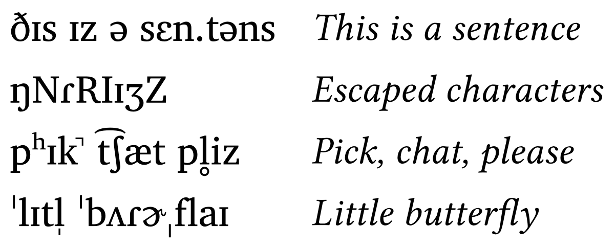
IPA transcription examples
#ipa("DIs \\s Iz \\s @ \\s sEn.t@ns")
#ipa("N \\N R \\R \\I I Z \\Z")
#ipa("p \\h I k \\* \\s \\t tS \\ae t \\s p \\r l iz")
You can download the sheet as a standalone file here.
2.2 Consonants
Two additional functions allow users to quickly create consonant tables and vowel trapezoids given a string of phonemes. The function #consonants() mirrors the pulmonic consonants table in the IPA chart with some minor changes. For example, affricates are shown when affricates: true, and the argument abbreviate: true shortens labels for both rows and columns. Figure 2 shows the consonant inventory for Italian.
Consonant table (Italian)
#consonants("italian", affricates: true, abbreviate: true)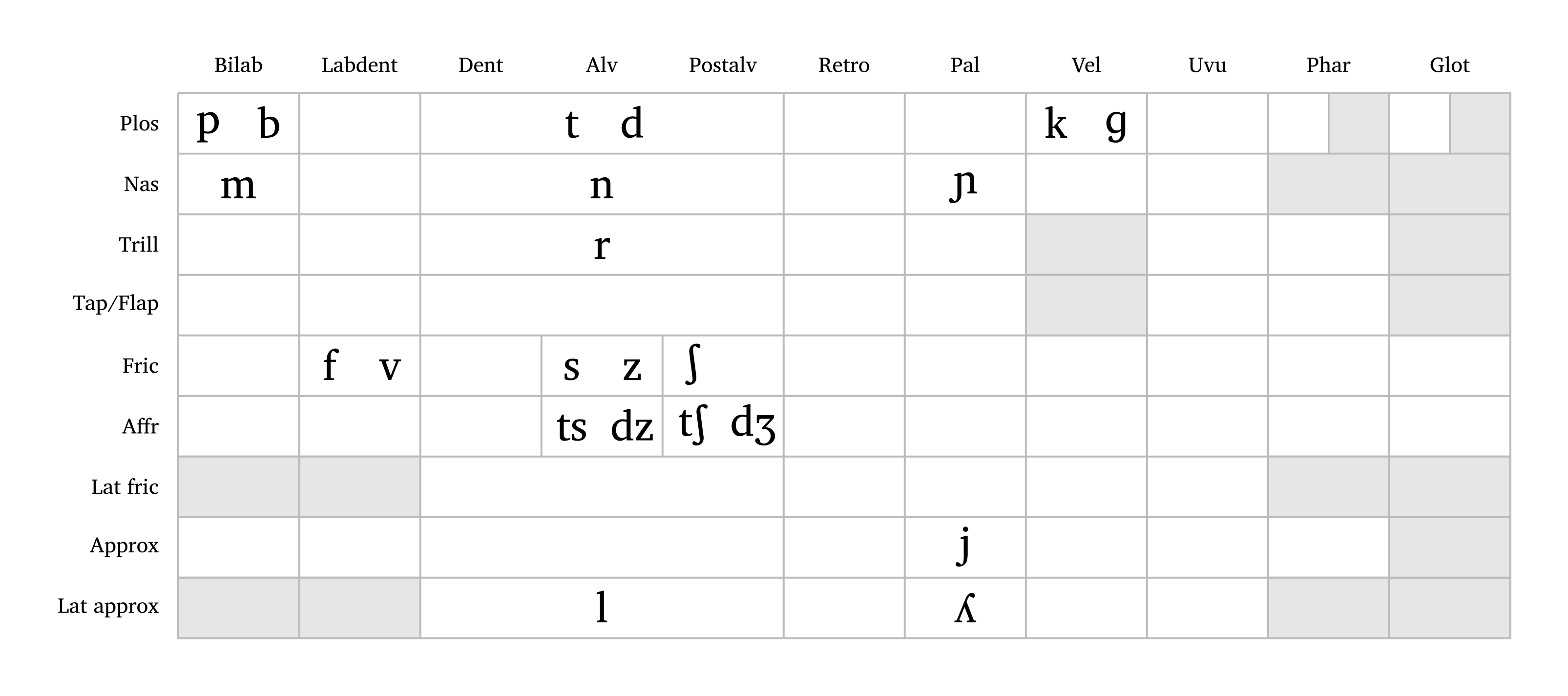
The user can either input a language name (Arabic, English, French, German, Italian, Japanese, Portuguese, Russian, Spanish — all lowercase; also all for all consonants) or a string of consonants to create a custom inventory. Custom consonants follow the same input format as #ipa(). Note that affricates and aspirated consonants require curly braces around them as well as affricates: true and aspirated: true, as shown in the caption of Figure 3. The function also supports flexible sizing with the scale argument.
Custom consonant table
#consonants("ts{ts}psS \\*r g{tS} {k \\h}", affricates: true, aspirated: true)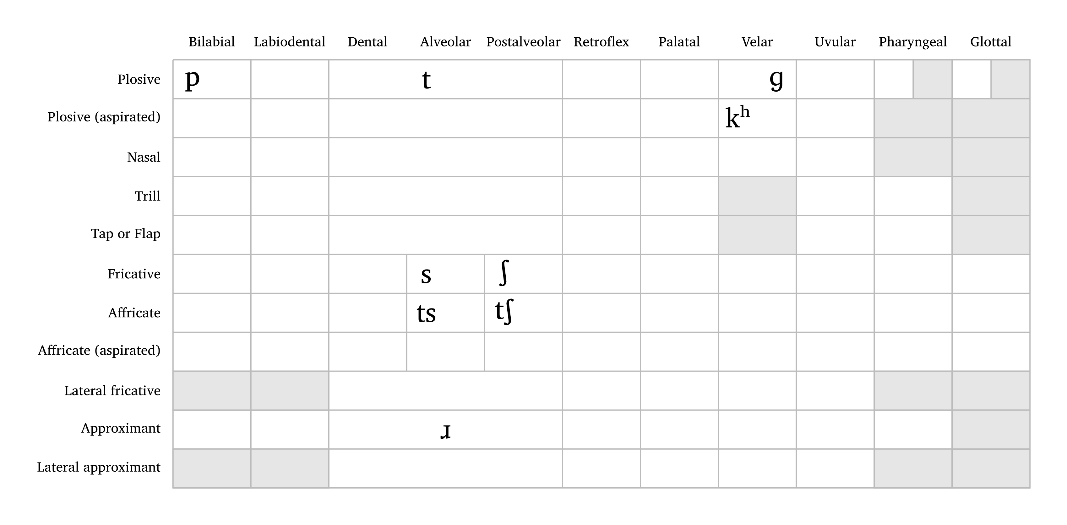
2.3 Vowels
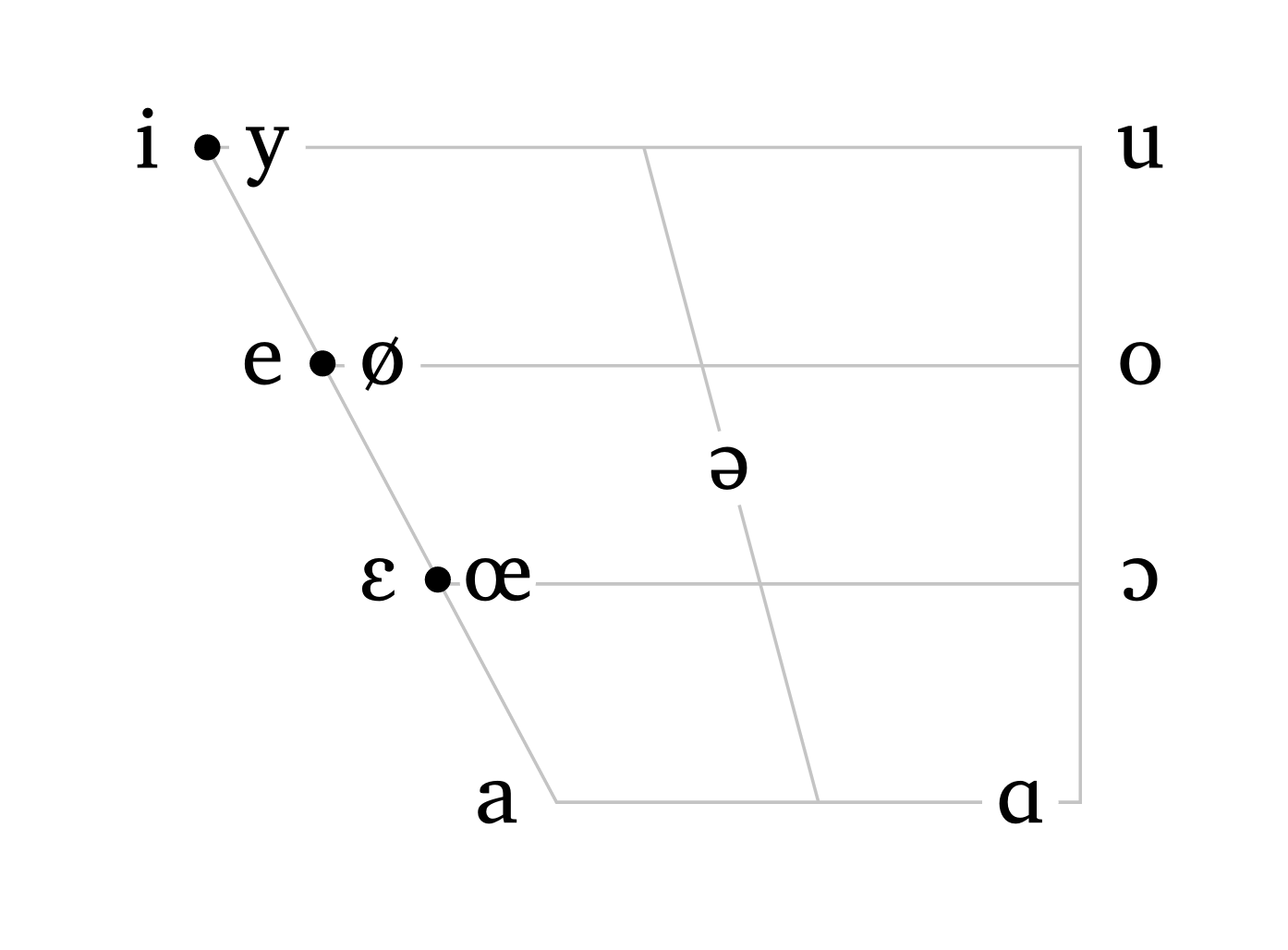
The function #vowels() also accepts either a pre-defined language or a string as input. The argument scale is available here too, so the user can adjust the size of the trapezoid as needed.
Vowel trapezoids
#vowels("english", scale: 0.6)
#vowels("french", scale: 0.6)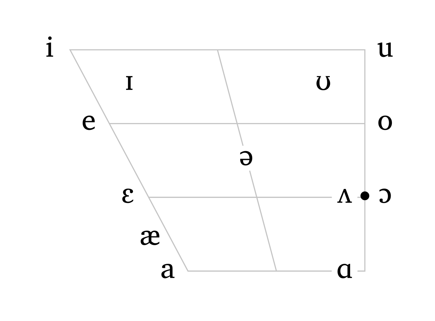
As of version 0.4.5, the function #vowels() accepts additional optional arguments to include arrows, shifted vowels, and highlights. Figure 6 illustrates how arrows and highlight can be used to display diphthongs in North American English. Arrows can be curved (curved: true) or dashed (arrow-style: "dashed"), and colors can be adjusted with arrow-color and highlight-color.
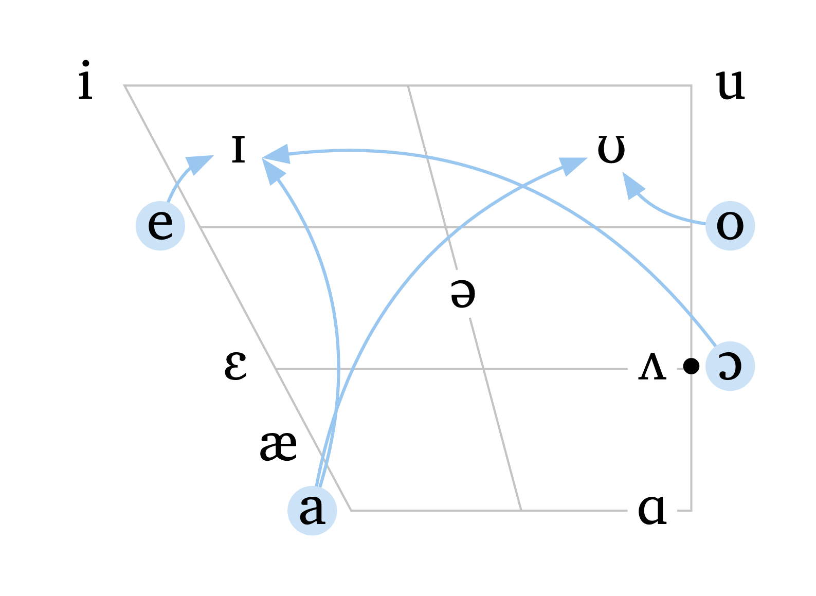
Vowels with arrows and highlights
#vowels(
   "english",
   arrows: (
     ("a", "U"),
     ("a", "I"),
     ("e", "I"),
     ("O", "I"),
     ("o", "U"),
   ),
   arrow-color: blue.lighten(60%),
   curved: true,
   highlight: ("a", "e", "o", "O"),
   highlight-color: blue.lighten(80%),
)
The argument shift allows you to specify a vowel as well as a shift from its original position, enabling much higher flexibility for illustrating dialectal variation. Shifted vowels can be independently targeted by highlight, and arrows can target shifted vowels using the same shifted values. The color and size of shifted vowels can be adjusted with shift-color and shift-size. Figure 7 demonstrates arrows, shifted vowels, and the option to remove grid lines (rows: 0 and cols: 0).
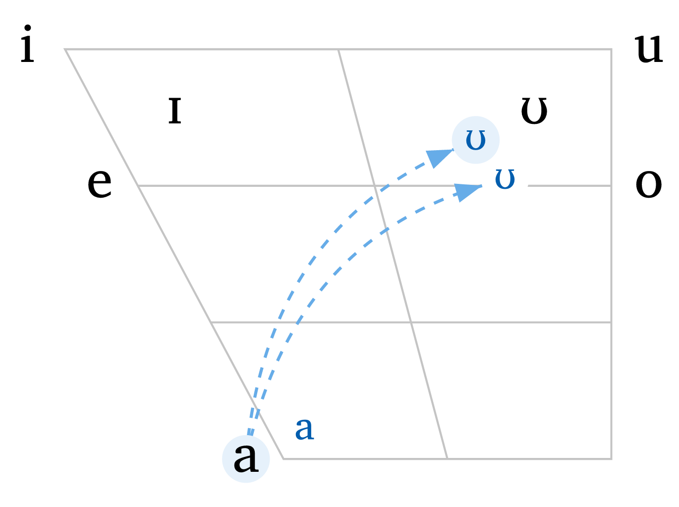
Vowels with shift
#vowels(
    "aeiouIU",
    arrows: (
      ("a", ("U", -0.6, -0.3)),
      ("a", ("U", -0.3, -0.7)),
    ),
    arrow-color: blue.lighten(40%),
    arrow-style: "dashed",
    curved: true,
    shift: (
      ("a", 0.6, 0.3),
      ("U", -0.6, -0.3),
      ("U", -0.3, -0.7),
    ),
    shift-size: 1.5em,
    shift-color: blue.darken(20%),
    highlight: ("a", ("U", -0.6, -0.3)),
    highlight-color: blue.lighten(90%),
  )
3 SPE
Rewrite rules can be complex, and phonokit provides two primitive functions for feature matrices that can be combined to form SPE-style rules (Chomsky and Halle 1968).
The first function is #feat-matrix(), which outputs the maximal feature matrix for a given phoneme (with the option for 0 values if all: true). This can be useful in introductory courses introducing the notion of distinctive features. The function is based on the features in Hayes (2009). Figure 8 shows matrices for the phonemes in “patchy”.
Feature matrices
#feat-matrix("p") #feat-matrix("\\ae") #feat-matrix("\\t tS") #feat-matrix("i")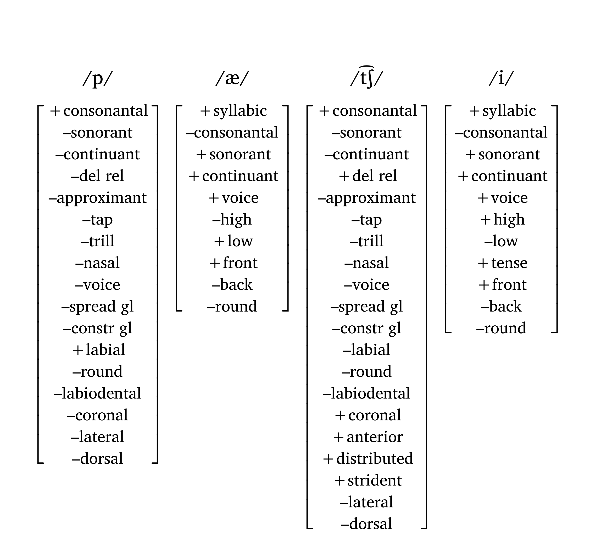
The second function, #feat(), creates a matrix given a set of features — this is the function used in a rewrite rule. Alpha notation requires a specific syntax: X + "feat" or X + [smallcaps("feat")]. A helper function #blank() adds a long underline for the context of application, and #a-r adds a right arrow (other arrows: #a-l, #a-u, #a-d, #a-lr, #a-ud, #a-sr, #a-sl, #a-r-large). Figure 9 shows a nasal place assimilation rule.
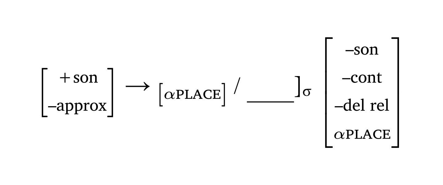
SPE rewrite rule
#feat("+son", "–approx") #a-r
  #feat(sym.alpha + [#smallcaps("place")]) / #blank()\]#sub[#sym.sigma]
  #feat("–son", "–cont", "–del rel", sym.alpha + [#smallcaps("place")])
4 Prosody
4.1 Sonority
When discussing the sonority principle in introductory courses, it is useful to illustrate relative sonority with a visual representation. The function #sonority(), based on the sonority scale in Parker (2011, 18), plots phonemes and their relative sonority profiles. If syllable boundaries are detected in the input, the function alternates between white and gray fills to distinguish each syllable.
Sonority profile
#sonority("vA \\*r .sI.ti", scale: 0.7)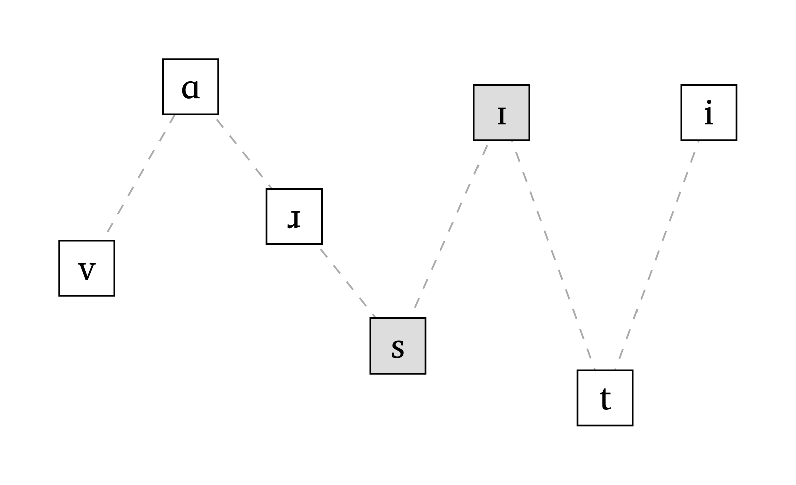
4.2 Syllables
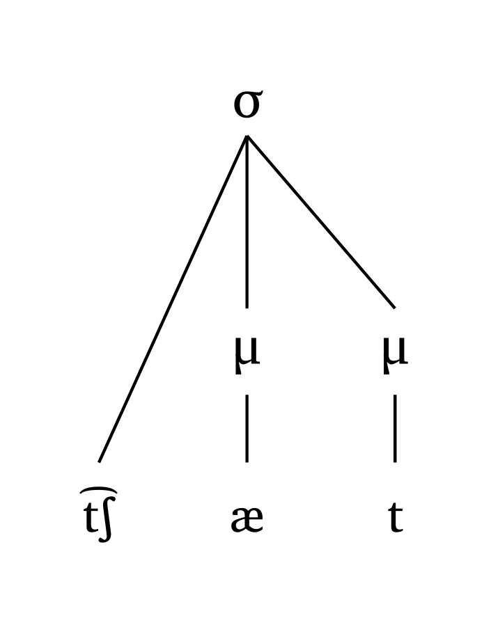
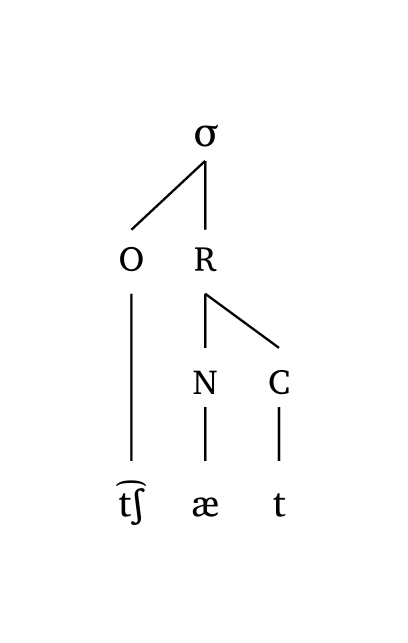
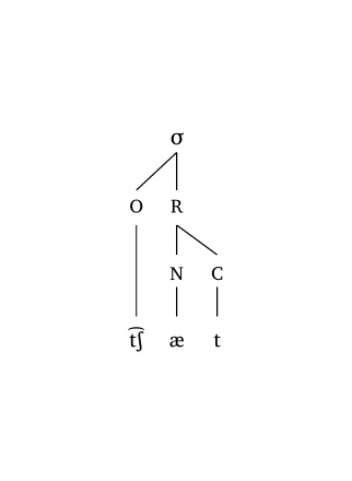
Two options are available: #syllable() for a classic onset-rhyme representation, and #mora(..., coda: true) for a moraic representation. The latter allows you to define whether codas project a mora (coda: true). Both functions are used for single-syllable representations only and accept the same #ipa() input conventions.
Syllable (onset-rhyme)
#syllable("\\t tS \\ae t")Syllable (moraic)
#mora("\\t tS \\ae t", coda: true)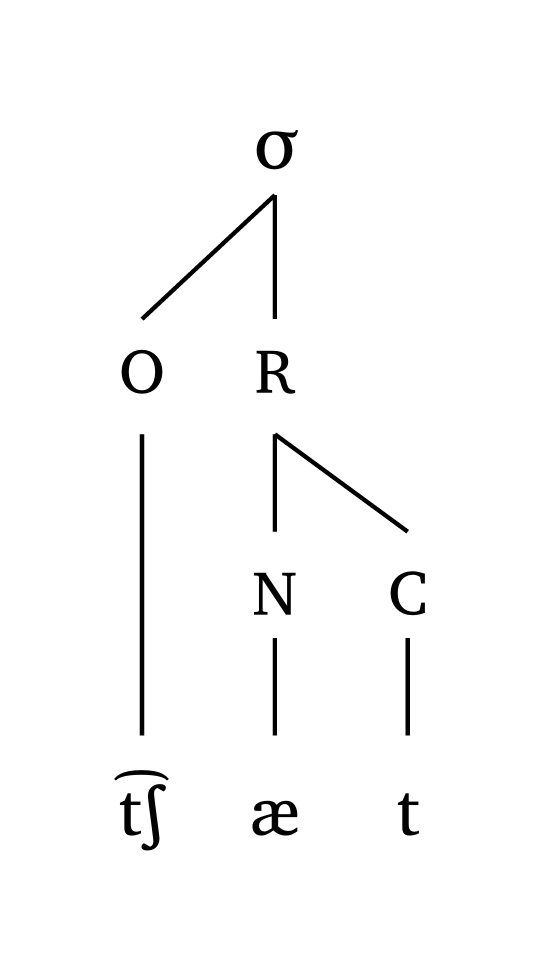
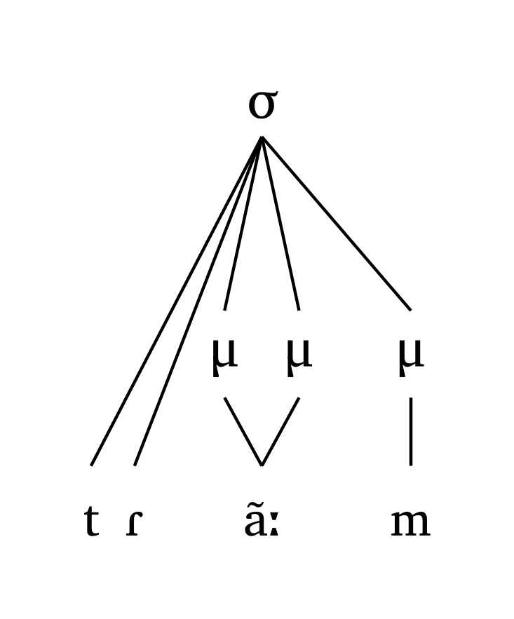
Vowel length is represented in both #syllable() and #mora(): the : character triggers the length mark, and in moraic representations two moras branch out of the vowel.
Long vowel, onset-rhyme
#syllable("tR \\~ a:m")Long vowel, moraic
#mora("tR \\~ a:m", coda: true)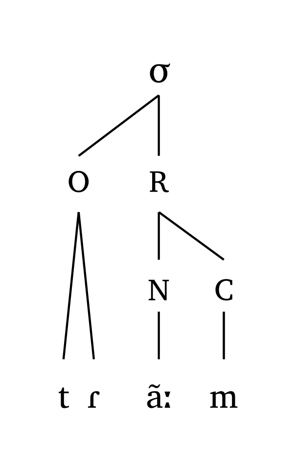
The dimensions adjust as a function of how many segments are found in the input. Figure 15 illustrates this with an extreme example.
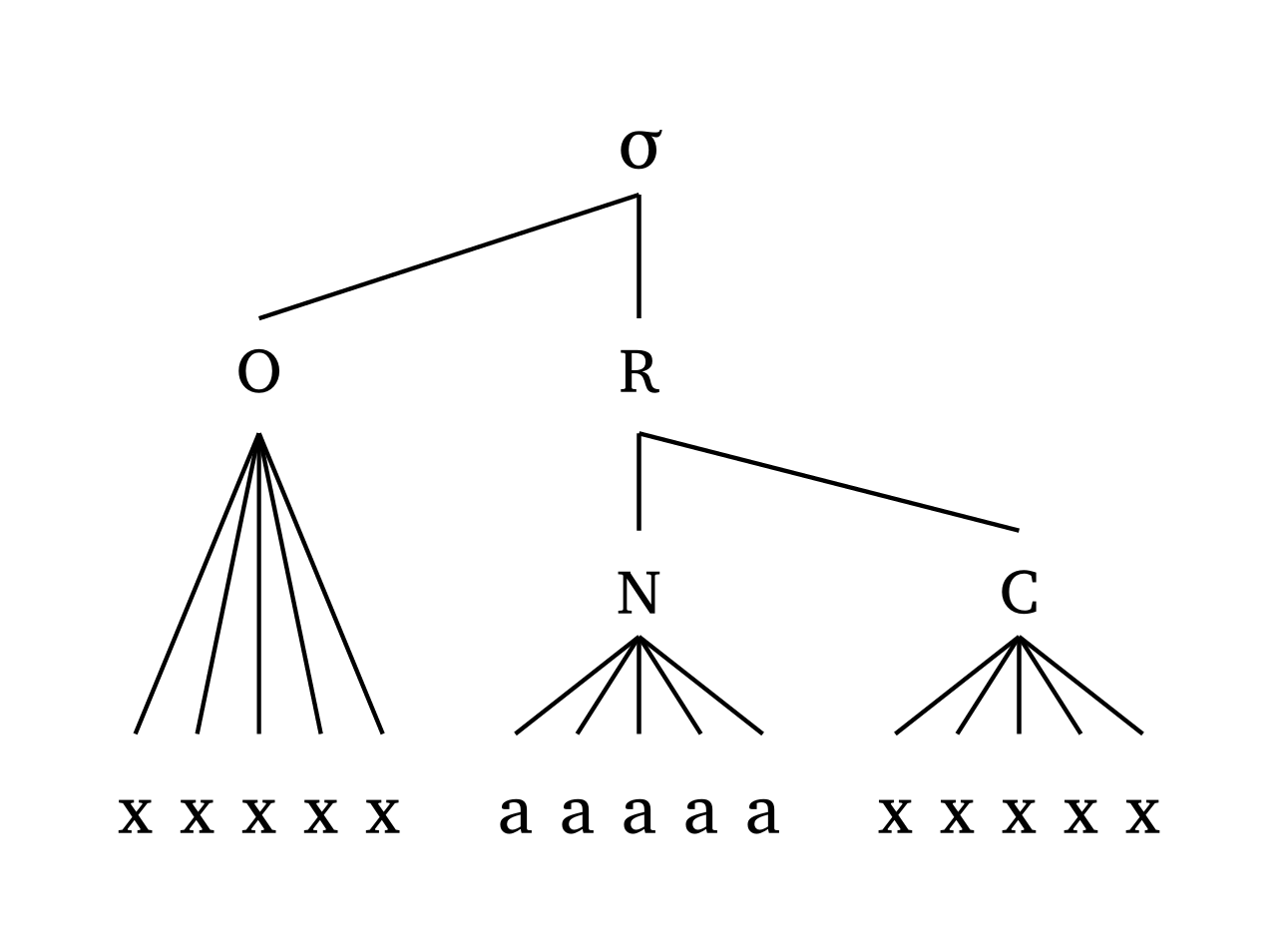
The scale argument takes care of both line width and text size uniformly. Figure 16, Figure 17, and Figure 18 show examples at different scale levels.

4.3 Feet
Yes. If you prefer “Ft” instead of \(\Sigma\), for example, see the Symbols appendix.
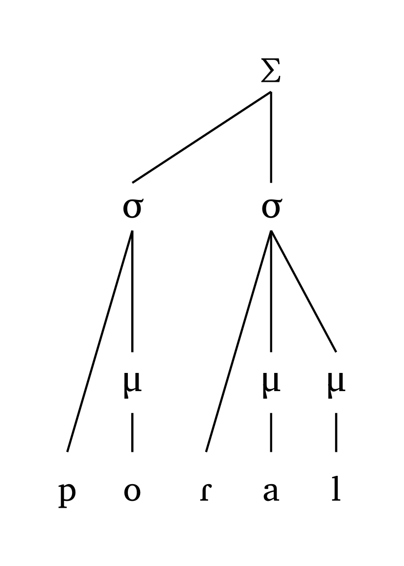
The functions #foot() and #foot-mora() handle a single foot. A period . indicates syllabification and a single apostrophe ' marks the head of the foot, allowing easy creation of trochees and iambs. Non-binary feet (dactyls, etc.) are also supported.
Trochee
#foot("'p \\h \\ae.\\*r Is")Iamb, moraic
#foot-mora("po.'Ral", coda: true)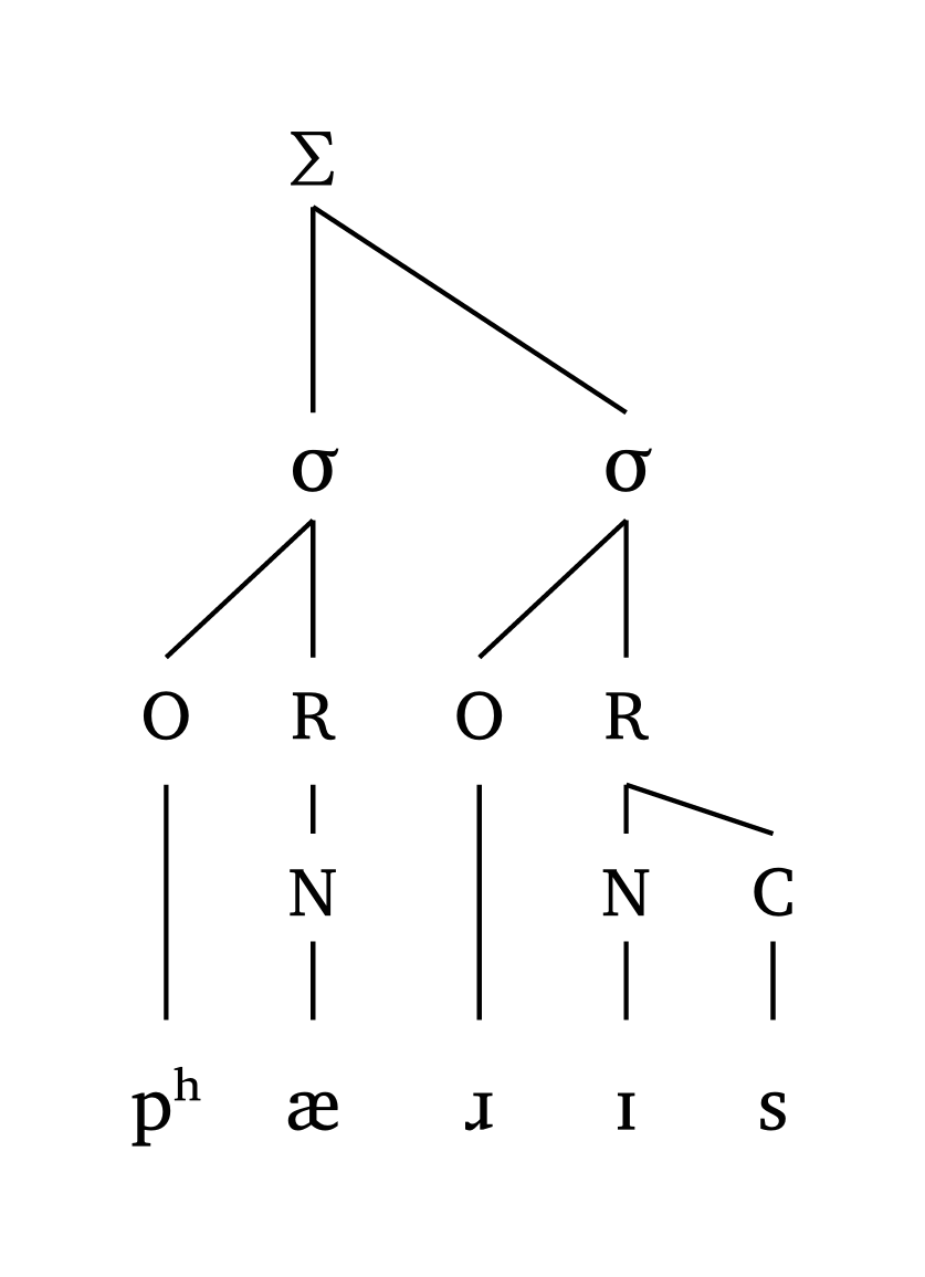
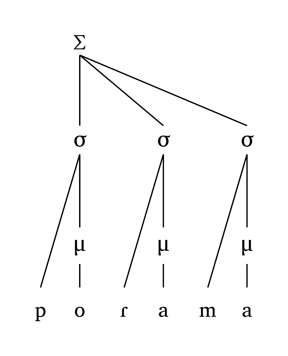
Dactylic foot
#foot("'po.Ra.ma")Dactylic foot, moraic
#foot-mora("'po.Ra.ma")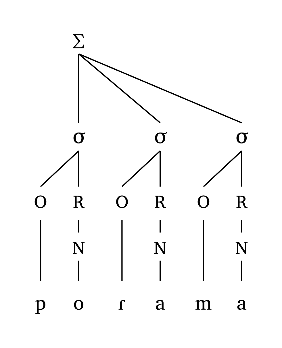
Geminates are also represented. In onset-rhyme representations, a geminate will be linked to the coda and the following onset. In moraic representations, coda: true provides the traditional representation.
Geminate, onset-rhyme
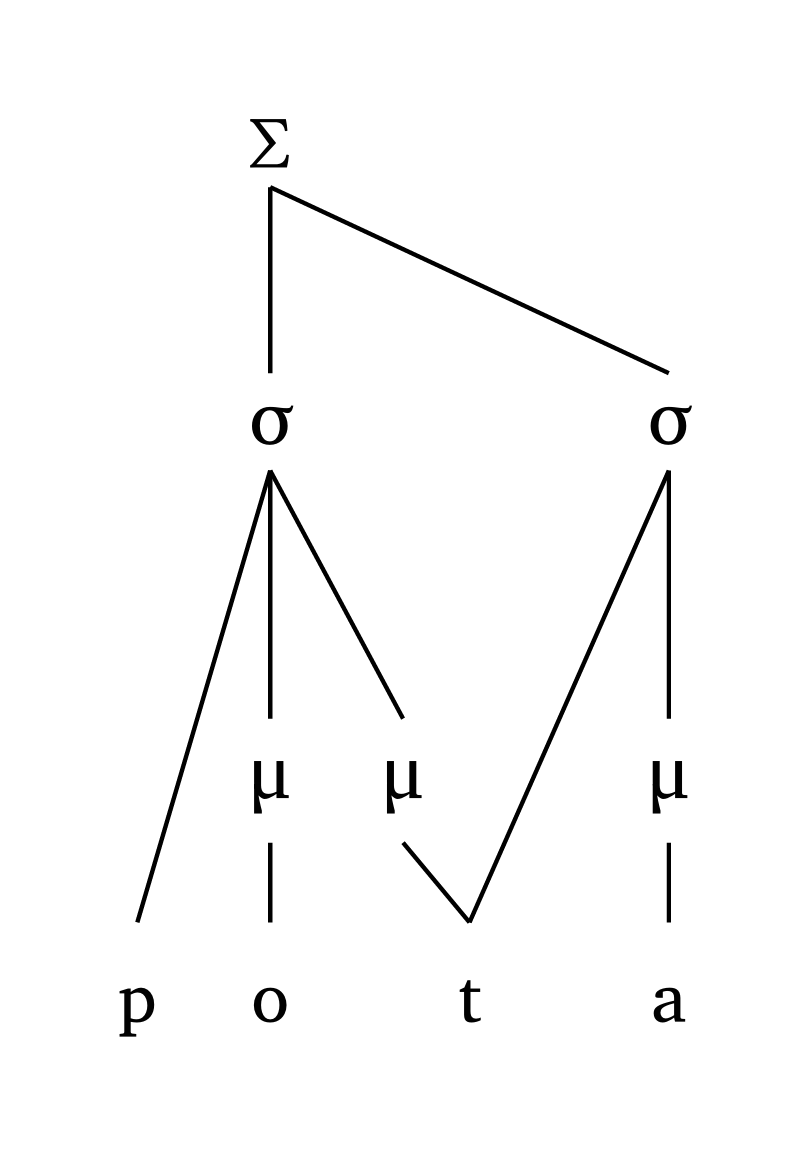
#foot("'pot.ta")Geminate, moraic
#foot-mora("'pot.ta", coda: true)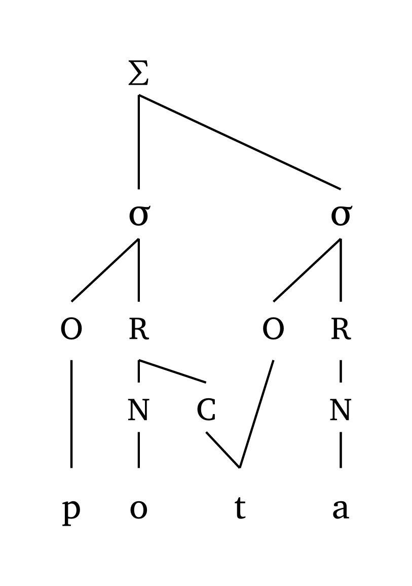
The height of \(\Sigma\) is proportional to the width of the representation to avoid superposition of lines in extreme cases, as Figure 25 demonstrates.
Extreme foot
#foot("'xa.xa.xa.xa.xa.xa.xa.xa.xa.xa.xa.xa", scale: 0.7)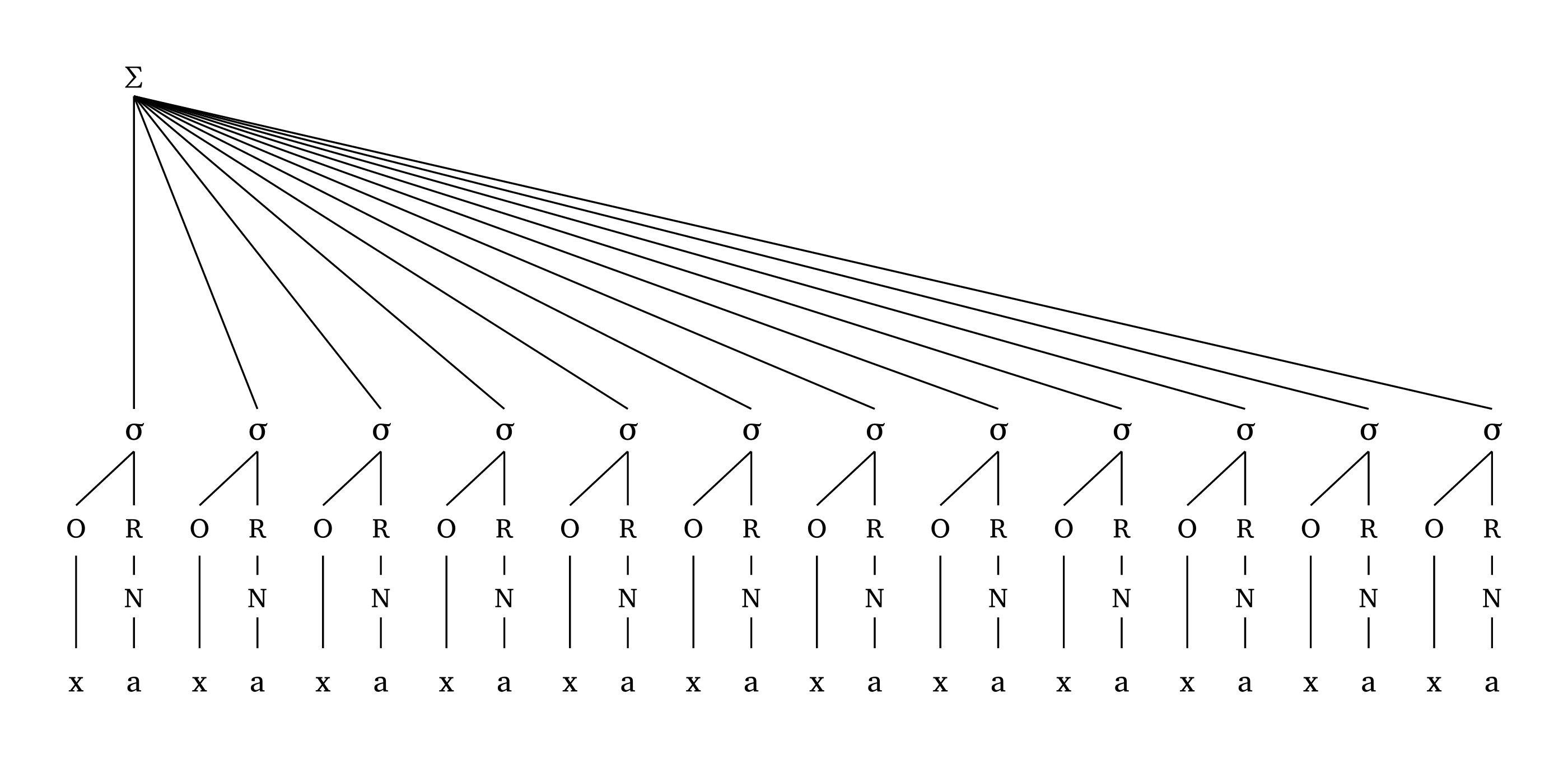
4.4 Prosodic words
Parentheses () define feet, so any syllable outside a foot is linked directly to the PWd. An apostrophe ' marks the head of each foot, and the argument foot: "R" or foot: "L" determines which foot carries primary stress in the word (when more than one foot is present).
Prosodic word (onset-rhyme)
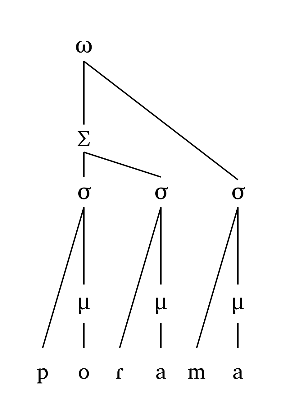
#word("('po.Ra).ma")Prosodic word (moraic)
#word-mora("('po.Ra).ma", coda: true)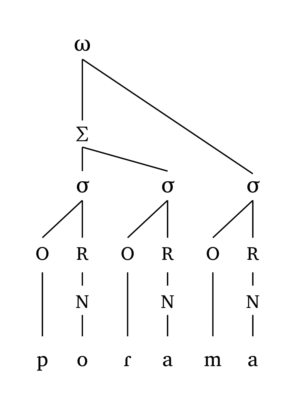
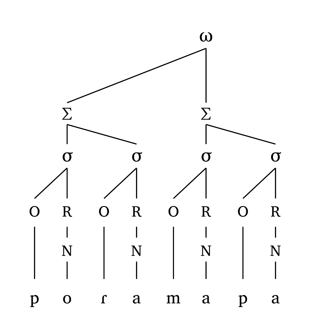
Two-foot PWd, left head
#word-mora("('po.Ra).('ma.pa)", foot: "L")Two-foot PWd, right head
#word("('po.Ra).('ma.pa)", foot: "R")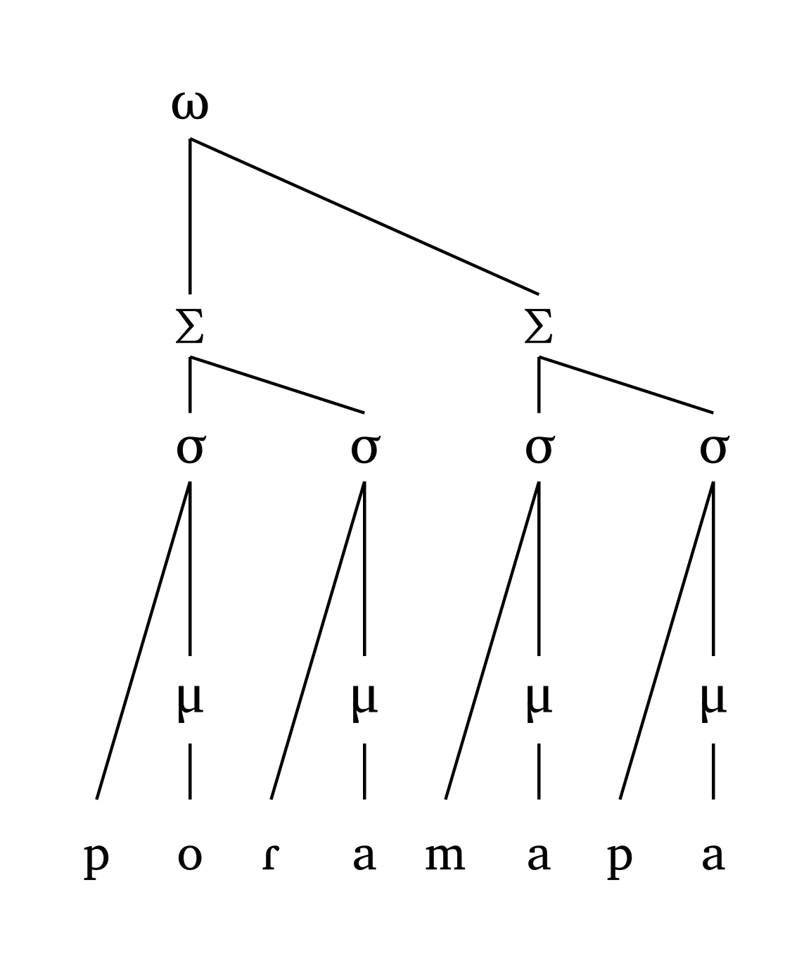
All lines are straight by design (no curved lines). In extreme scenarios — e.g., where an unfooted syllable is very far from the head foot — the height is adjusted to avoid line crossings, as Figure 30 demonstrates.
Extreme PWd
#word("xa.(xa.xa)(xa.xa)(xa.xa)(xa.xa)", scale: 0.7)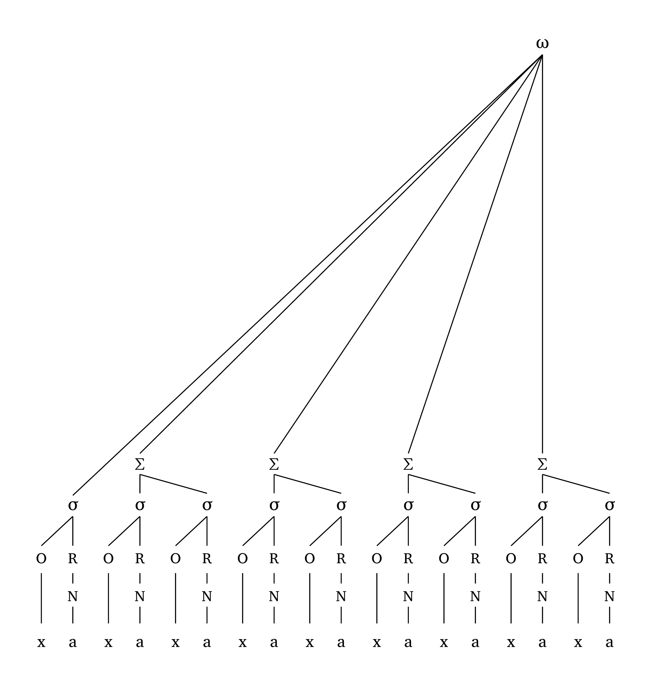
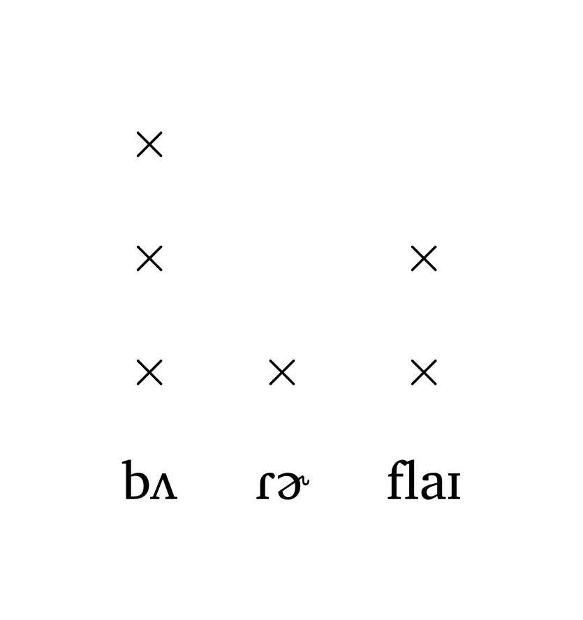
4.5 Metrical grid
The function #met-grid() creates a metrical grid using \(\times\) to indicate prominence. The goal is high-quality output with minimal effort. Figure 31 and Figure 32 show grids for the word butterfly.
Metrical grid (string input)
#met-grid("bu3.tter1.fly2")Metrical grid (tuple/IPA input)
#met-grid(("b2", 3), ("R \\schwar", 1), ("flaI", 2))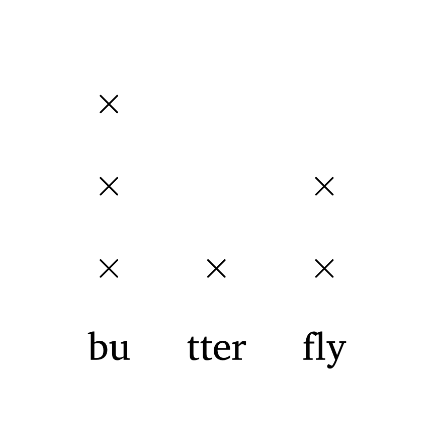
5 Autosegments
The function #autoseg() allows you to represent either features or tones on a separate tier, including linking, delinking, floating tones, and contour tones. Inputs are arrays, so each phoneme is entered individually. This allows for empty spaces, domain boundary symbols, etc.
5.1 Feature spreading
Figure 33 demonstrates #autoseg() in a simple scenario of feature spreading. The argument links is an array of tuples: ((2,1),) means “draw a link from index 2 to index 1”. The argument arrow adds or removes arrow heads on linking lines.
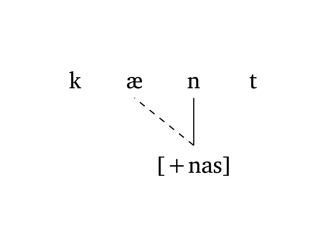
Nasal spreading
#autoseg(
    ("k", "\\ae", "n", "t"),
    features: ("", "", "[+nas]", ""),
    links: ((2, 1),),
    spacing: 1.0,
    arrow: false,
  )
Figure 34 shows an example of metaphony in Brazilian Veneto (Garcia and Guzzo 2023) where [+high] spreads from the final /i/ to /e/ (position 3) and /o/ (position 1). The argument gloss allows quick annotation.
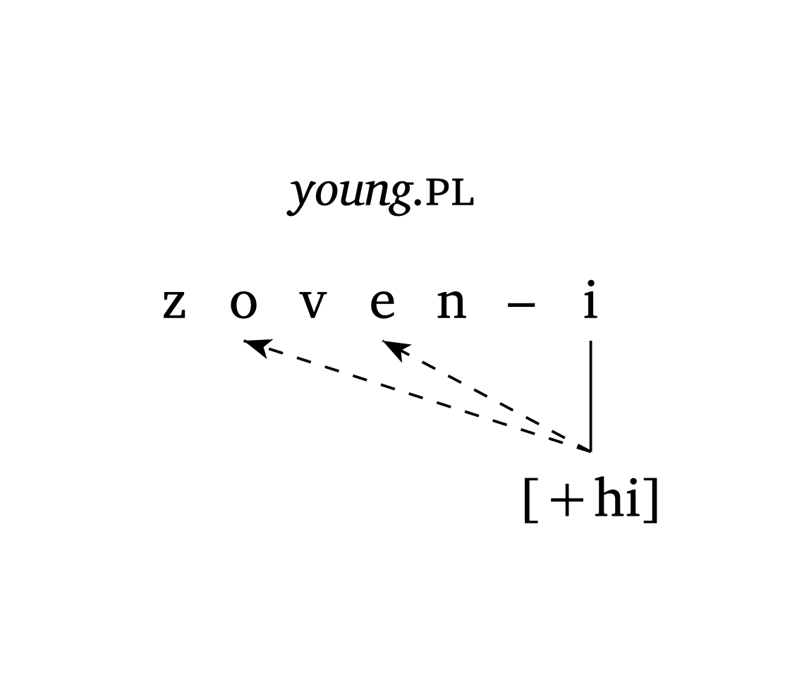
Metaphony (Brazilian Veneto)
#autoseg(
    ("z", "o", "v", "e", "n", "–", "i"),
    features: ("", "", "", "", "", "", "[+hi]"),
    links: ((6, 3), (6, 1)),
    spacing: 0.5,
    arrow: true,
    gloss: [_young_#smallcaps(".pl")],
  )
5.2 Tones
The argument tone: true “flips” the representation vertically to show tones above the segmental tier. Figure 35 shows low tone spreading without delinking in Nupe (Zsiga 2024).
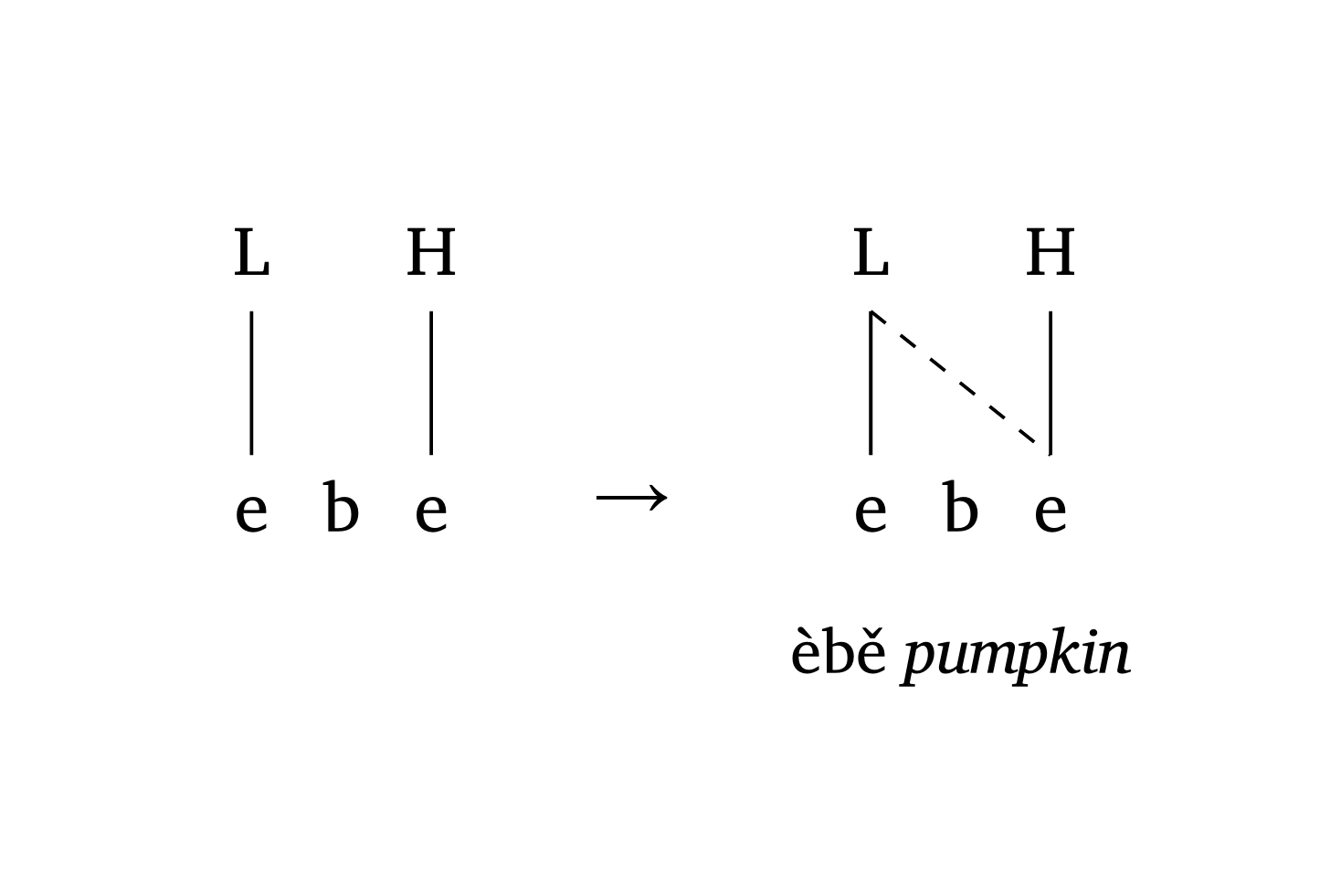
Tone spreading (Nupe)
#autoseg(
  ("e", "b", "e"),
  features: ("L", "", "H"),
  spacing: 0.5,
  tone: true,
  gloss: [],
)
#a-r  // arrow between stages
#autoseg(
  ("e", "b", "e"),
  features: ("L", "", "H"),
  links: ((0, 2),),
  spacing: 0.5,
  tone: true,
  gloss: [èbě _pumpkin_],
)
Floating tones can be added with the float argument. Figure 36 demonstrates how to add a floating tone and draw a circle around it with the highlight argument.
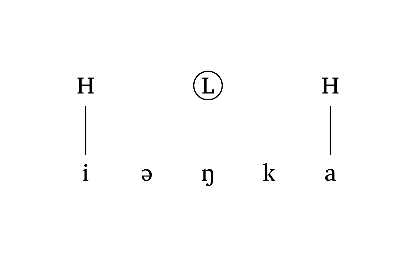
Floating tone
#autoseg(
      ("i", "@", "N", "k", "a"),
      features: ("H", "", "L", "", "H"),
      highlight: (2,),
      spacing: 1.0,
      tone: true,
      float: (2,),
    )
Spreading from a contour tone requires a tuple inside features for the vowel linked to two tones. The links argument uses nested tuples: (((2, 0), 1),) means “from the first tone at position 2 (i.e., H), draw a dashed line to segment 1”. Figure 37 illustrates this.
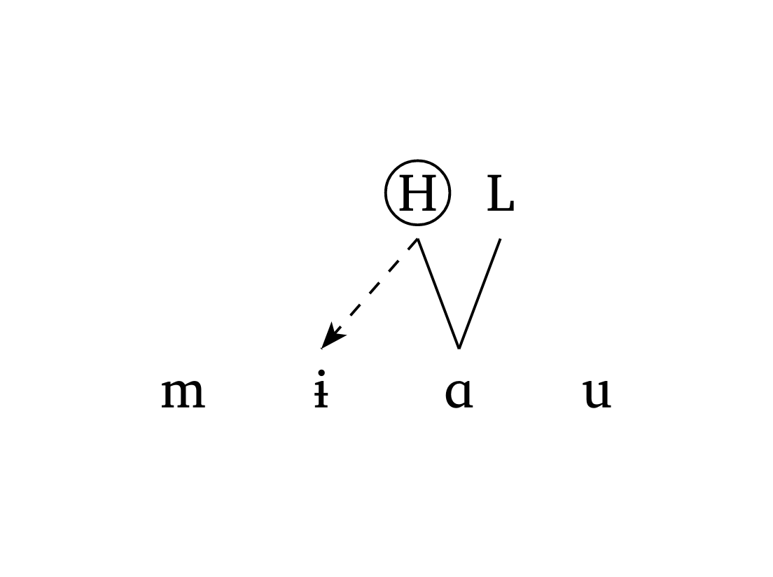
Contour tone
#autoseg(
  ("m", "1", "A", "u"),
  features: ("", "", ("H", "L"), ""),
  links: (((2, 0), 1),),
  tone: true,
  highlight: ((2, 0),),
  spacing: 1.0,
  arrow: true,
),
Figure 38 shows a three-stage OCP effect in Vai (Zsiga 2024), demonstrating delinking (delinks) and one-to-many tone relationships (multilinks). The argument delinks: ((3, 3),) states that the link between position 3 and itself must be delinked. The argument multilinks: ((6, (6, 9)),) means “center a tone on segments 6 and 9 simultaneously”.
OCP effects (Vai)
#autoseg(
      ("m", "u", "s", "u"),
      features: ("", "L", "", "H"),
      tone: true, spacing: 0.5, baseline: 37%,
      gloss: [_woman_],
    ) +
    #autoseg(
      ("k", "u", "n", "d", "u"),
      features: ("", "H", "", "", ""),
      tone: true,
      float: (1,),
      multilinks: ((1, (1, 4)),),
      spacing: 0.5, baseline: 37%,
      arrow: false,
      gloss: [_short_],
    ) #a-r
    #autoseg(
      ("m", "u", "s", "u", "–", "k", "u", "n", "d", "u"),
      features: ("", "L", "", "H", "", "", "H", "", "", ""),
      links: ((1, 3),),
      delinks: ((3, 3),),
      arrow: false,
      multilinks: ((6, (6, 9)),),
      tone: true,
      baseline: 37%,
      spacing: 0.50,
      gloss: [_short woman_],
    )
5.3 Prosody with ToBI
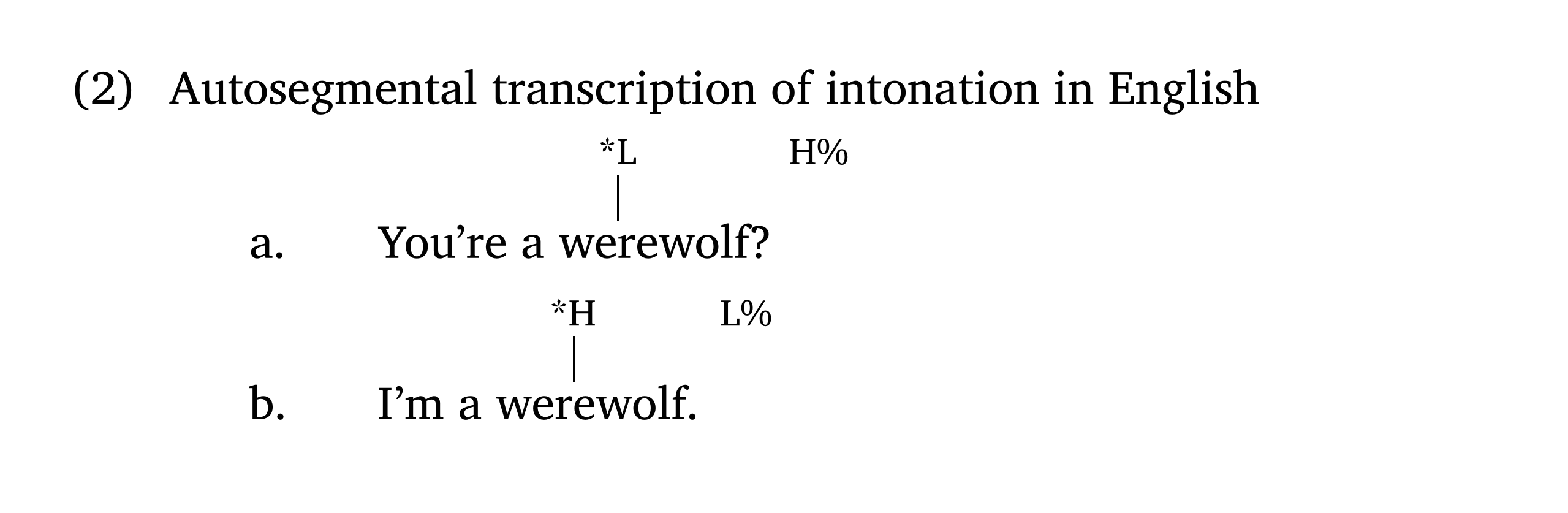
Adding ToBI labels to strings can be achieved with the function #int(). The argument line: false turns off the vertical stem (e.g., for boundary tones). By default, the font size of tones is 0.8em.
Inline ToBI
You're a we#int("*L")rewolf?#h(2em)#int("H%", line: false)

I'm a wer#int("*H")ewolf.#h(2em)#int("L%", line: false)
Note that #int() is not meant to be used in numbered/unnumbered lists. In the vast majority of cases, strings with ToBI labels will appear in numbered examples — see the Numbered examples section.
5.4 Multi-tier
The function #multi-tier() provides the freedom to create a wide range of non-linear structures that cannot be generated by single-purpose functions. The main argument is levels, an array of rows, where each row is an array of elements. Elements are automatically linked to the element on the level below; additional links can be specified with the links argument.
Figure 40 reproduces a figure from Booij (2012, 159) on the interface of phonology and morphology. Figure 41 shows the same figure with show-grid: true to help visualize positions.
Multi-tier (morphophonology)
#multi-tier(
  show-grid: true, // <- to help you see the grid
  levels: (
    ("", "", "", "", ("Adj", 3.5)),
    ("", "", "", "", ("Adj", 3.5)),
    ("", ("Af", 0.5), "", ("N", 2.5), "Af"),
    ("in", "ter", "na", "tion", "al"),
    ("sigma", "sigma", "sigma", "sigma", "sigma"),
    ("Sigma", "", "Sigma", "", ""),
    ("", "", "omega", "", ""),
  ),
  links: (
    ((0, 4), (2, 1)), // Adj -> Af
    ((1, 4), (2, 3)), // Adj -> N
    ((2, 1), (3, 0)), // Af -> in
    ((2, 3), (3, 2)), // N -> na
    ((5, 0), (4, 1)), // Ft -> Syl
    ((5, 2), (4, 3)), // Ft -> Syl
    ((6, 2), (5, 0)), // PWd -> Ft
    ((6, 2), (4, 4)), // PWd -> Ft
  ),
)
Elements specified as ("N", 2.5) are placed at fractional positions on the grid. The function also automatically detects Greek letters: adding "sigma" renders as \(\sigma\), "Sigma" as \(\Sigma\), "omega" as \(\omega\). Numbers in elements are automatically rendered as subscripts.
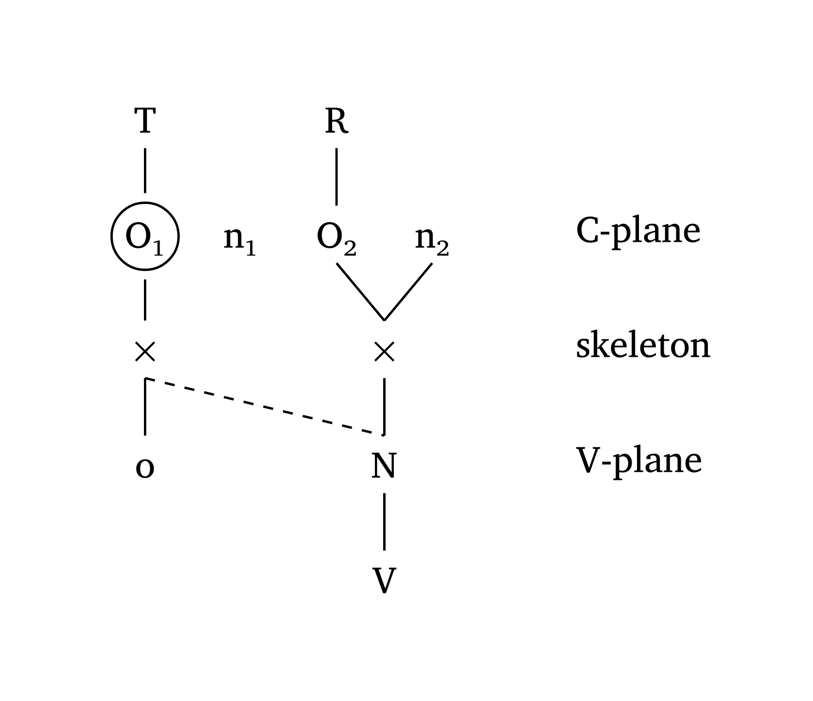
#multi-tier() can also create Government Phonology and CV Phonology representations. Figure 42, adapted from Goad (2012, 355), shows how arrows and arrow-delinks work. It is also possible to label tiers, as shown in Figure 43, adapted from Carvalho (2017).
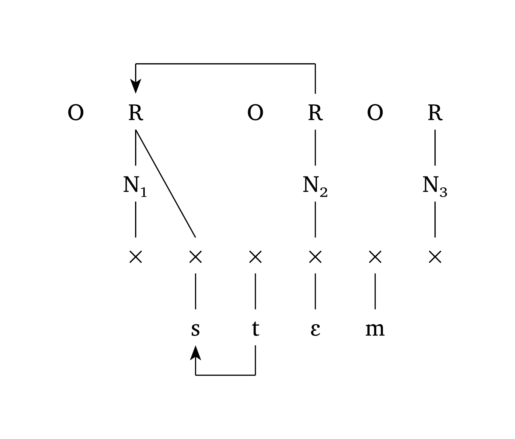
Government Phonology
#multi-tier(
  levels: (
    ("O", "R", "", "O", "R", "O", "R"),
    ("", "N1", "", "", "N2", "", "N3"),
    ("", "x", "x", "x", "x", "x", "x"),
    ("", "", "s", "t", "E", "m", ""),
  ),
  links: (((0, 1), (2, 2)),),
  ipa: (3,),
  arrows: (
    ((3, 3), (3, 2)),
    ((0, 4), (0, 1)),
  ),
  arrow-delinks: ((1,)),
  spacing: 1,
)
CV Phonology with tier labels
#multi-tier(
  levels: (
    ("T", "", "R", ""),
    ("O1", "n1", "O2", "n2"),
    ("x", "", ("x", 2.5), ""),
    ("o", "", ("N", 2.5), ""),
    ("", "", ("V", 2.5), ""),
  ),
  links: (((1, 3), (2, 2)),),
  dashed: (((2, 0), (3, 2)),),
  level-spacing: 1.2,
  highlight: ((1, 0),),
  spacing: 1,
  stroke-width: 0.7pt,
  tier-labels: (
    (1, "C-plane"),
    (2, "skeleton"),
    (3, "V-plane"),
  ),
  scale: 1,
)
6 Feature geometry
Feature geometry presents some important challenges, including the user interface: if too many degrees of freedom are available, a function becomes too convoluted. phonokit offers two dedicated functions: #geom() for single-segment trees and #geom-group() for multiple trees and processes.
6.1 Single trees
The arguments of #geom() are named after the nodes they add. If you add a node \(n\), the function automatically builds any parent node needed. For example, adding voice: true also adds [laryngeal]; adding anterior: true also adds [coronal]. Arguments accept both boolean and string values: nasal: true adds [nasal], while nasal: "+" adds [+nasal].
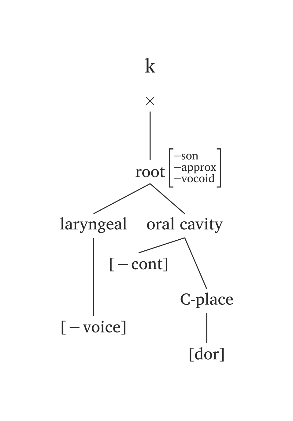
Figure 44 reproduces the full consonant representation from Clements and Hume (1995, 292).
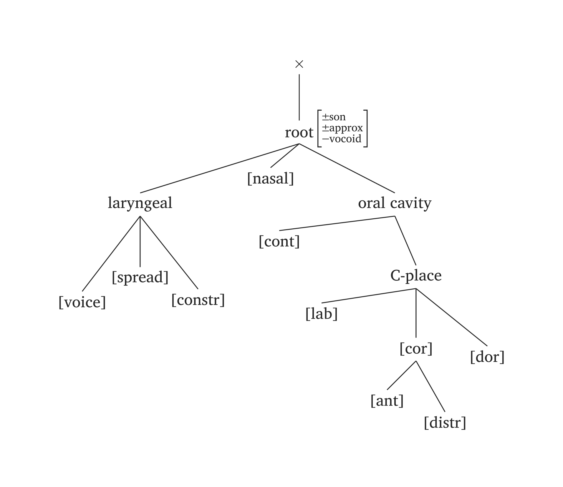
Full consonant feature geometry
#geom(
root: ("±son", "±approx", "-vocoid"),
spread: true,
constricted: true,
nasal: true,
voice: true,
labial: true,
anterior: true,
distributed: true,
dorsal: true,
continuant: true,
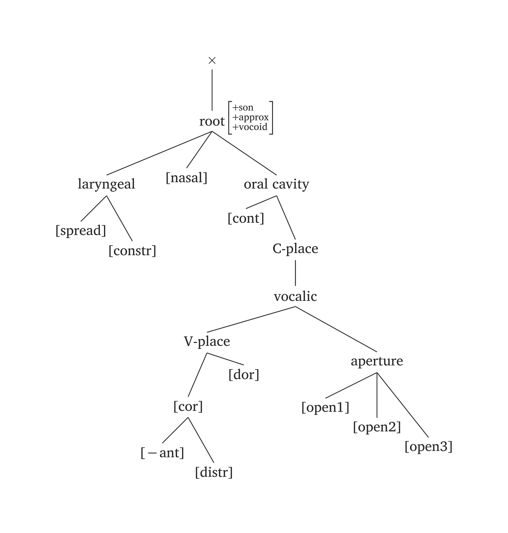
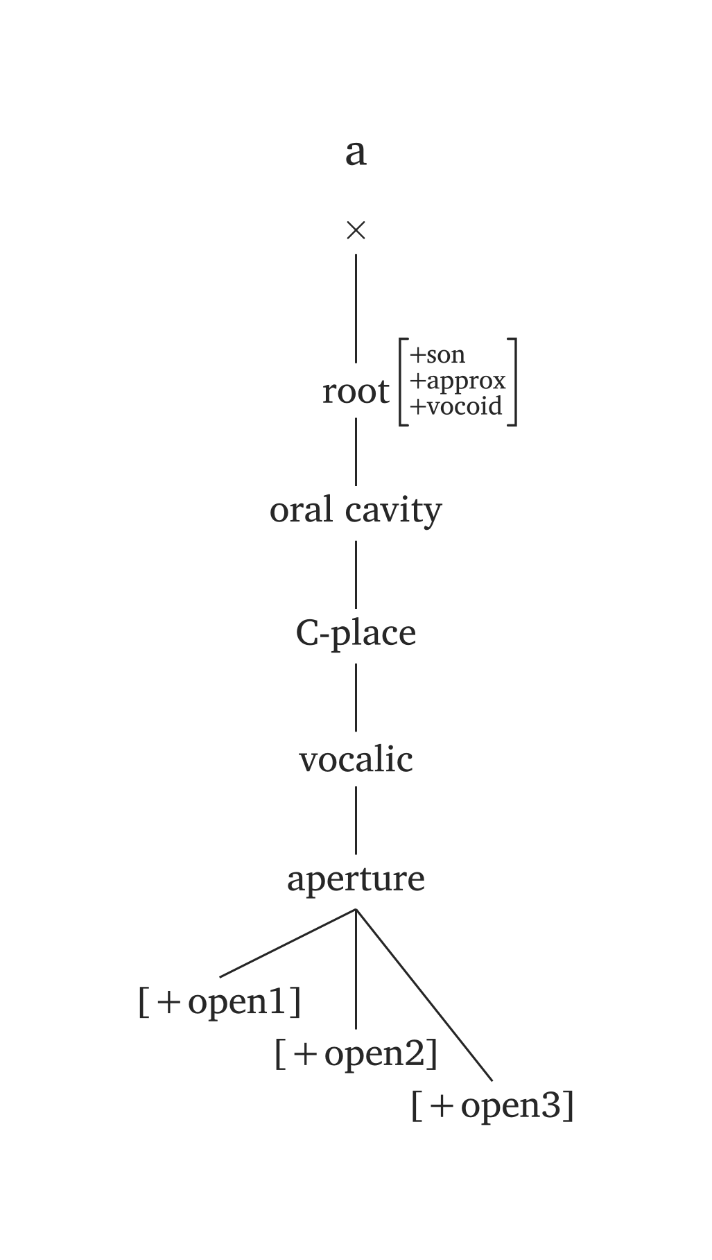
)Full vocoid feature geometry
#geom(
  root: ("+son", "+approx", "+vocoid"),
  spread: true,
  constricted: true,
  nasal: true,
  vplace: true,
  aperture: (true, true, true),
  coronal: true,
  anterior: "-",
  distributed: true,
  dorsal: true,
  continuant: true,
  scale: 0.9,
)
Several phonemes come pre-built in #geom() via the ph argument, using the same #ipa() conventions. In the figures below, the only code needed is #geom(ph: "..."). You will also note timing units added by default (x). You can disable timing units by adding timing: false, or you can add morae instead (timing: "mora" or timing: "mu"). The timing argument also takes an array for long vowels: timing: ("x", "x"). For example, if you prefer morae to x slots, you’d add timing: ("mora", "mora") for the long vowel in Figure 47.
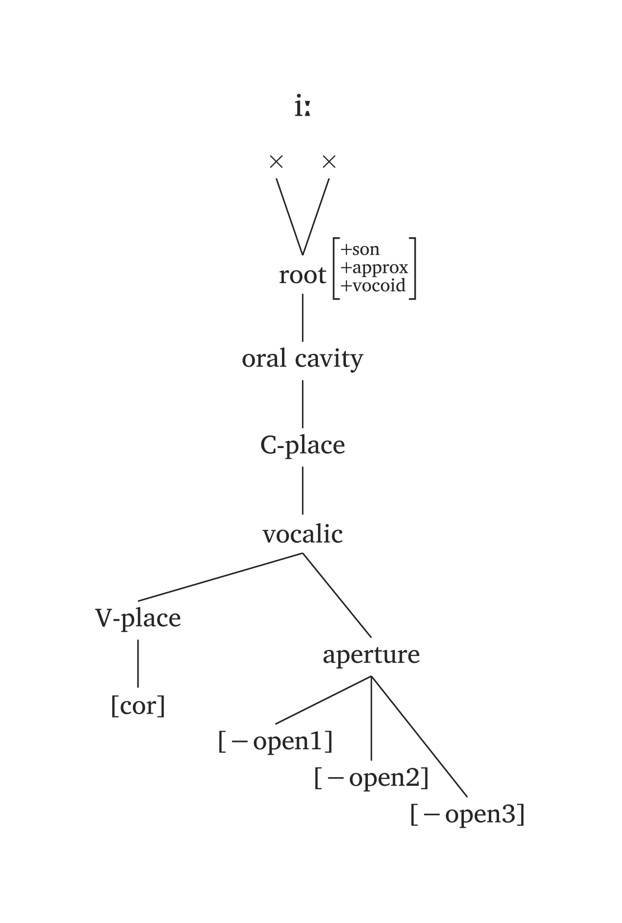
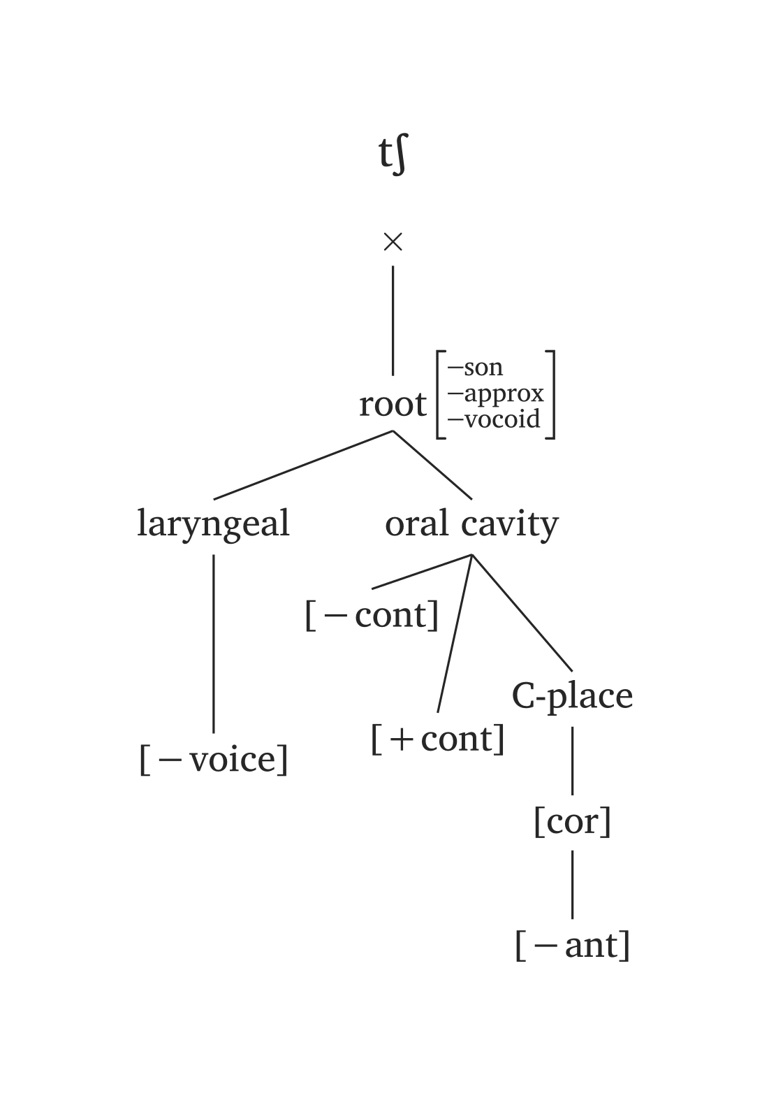
The ph argument offers minimal syntax, but you are not locked to presets. Any node can be overridden: for example, #geom(ph: "a", aperture: (true,)) overrides only the aperture specification for the preset /a/.
6.2 Multiple trees
The function #geom-group() works as a wrapper to “glue” multiple #geom() trees together, enabling arrows across trees. The key additional arguments are arrows, curved, and delinks.
Arrows reference nodes by name with a tree index: "nasal2" refers to [nasal] in tree 2, "root1" to the root in tree 1. The argument ctrl adjusts the control points of the Bezier curve (start and end directions). Figure 50 shows the spreading of [nasal].
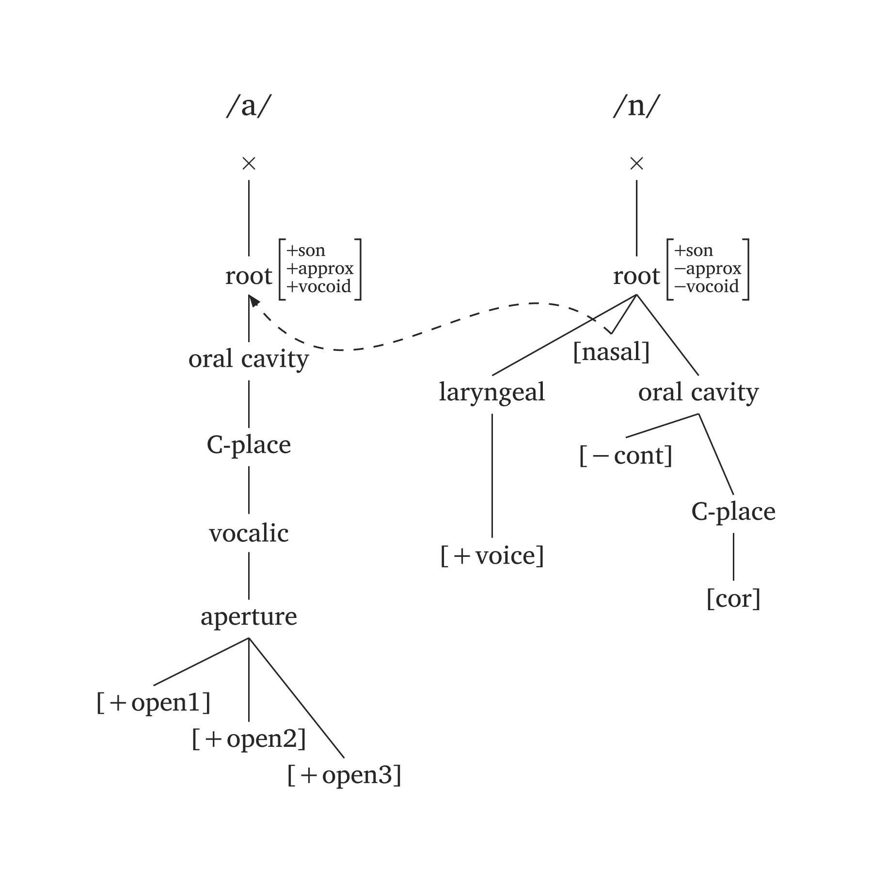
Nasalization
#geom-group(
(ph: "/a/"),
(ph: "/n/"),
arrows: (
(from: "nasal2",
to: "root1",
ctrl: (1.1, -1.5)),
),
curved: true,
gap: 1,
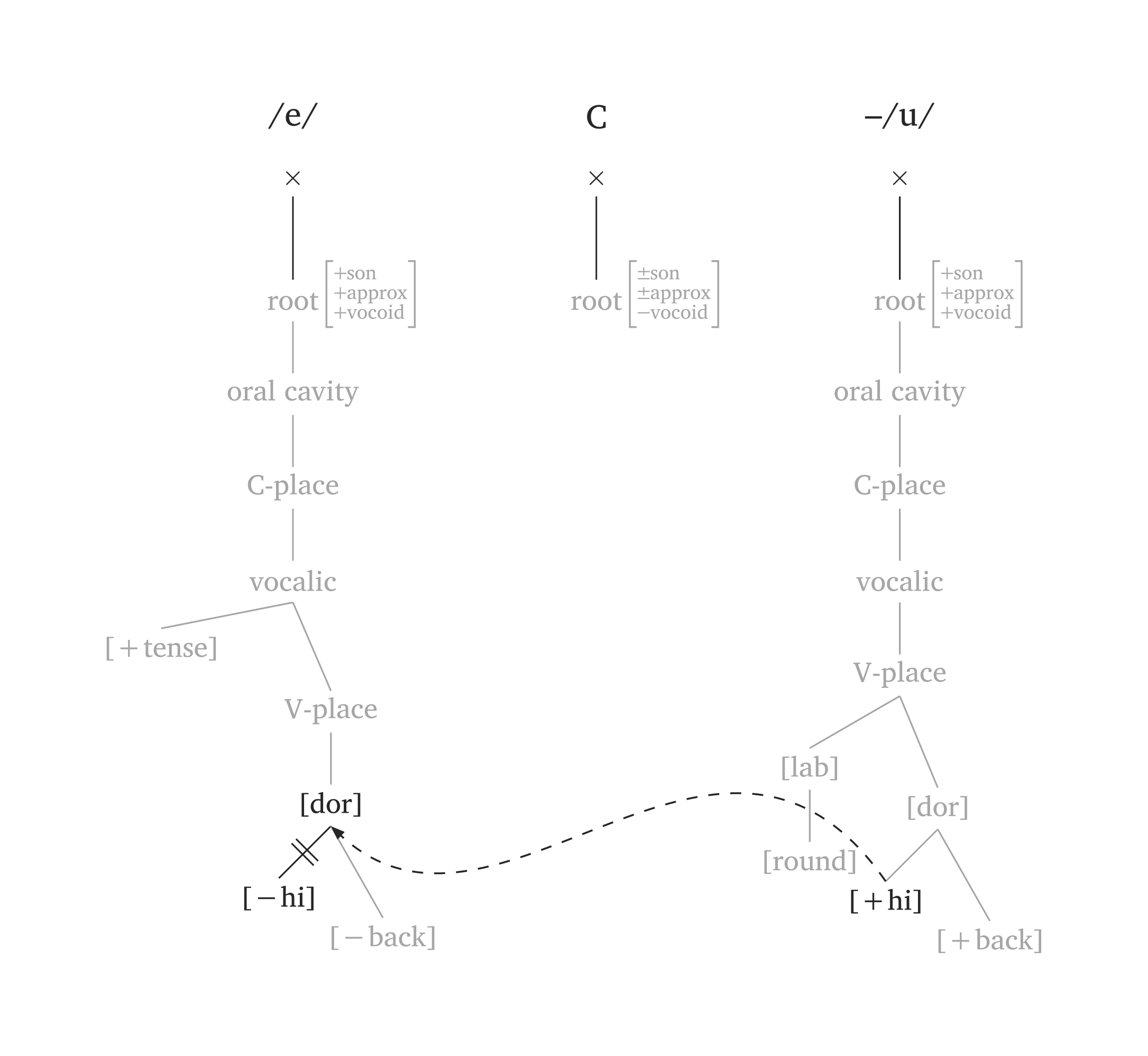
)By default, #geom() uses the Clements and Hume (1995) model. Setting model: "sagey" uses height features (Sagey 1986) instead of aperture. The argument highlight dims the entire representation and only highlights the specified nodes. Figure 51 illustrates metaphony where /e/ → [i] / __ C₀ /u/:
Metaphony (Sagey model)
#geom-group(
  (ph: "/e/"),
  (ph: "\\C"),
  (ph: "/u/", prefix: "-"),
  arrows: (
    (from: "high3", to: "dorsal1", ctrl: (2.3, -1.5)),
  ),
  delinks: ("high1",),
  highlight: ("high1", "dorsal1", "high3"),
  gap: 1.5,
  model: "sagey",
)
7 Optimality Theory
The function #tableau() generates OT tableaux (Prince and Smolensky 1993). It takes six arguments: input, candidates, constraints, violations, winner, and dashed-lines. The violations argument requires a nested structure. The winner candidate counts from zero. Cells are automatically shaded after a fatal violation (!), and the pointing finger symbol ☞ is added for the winner.
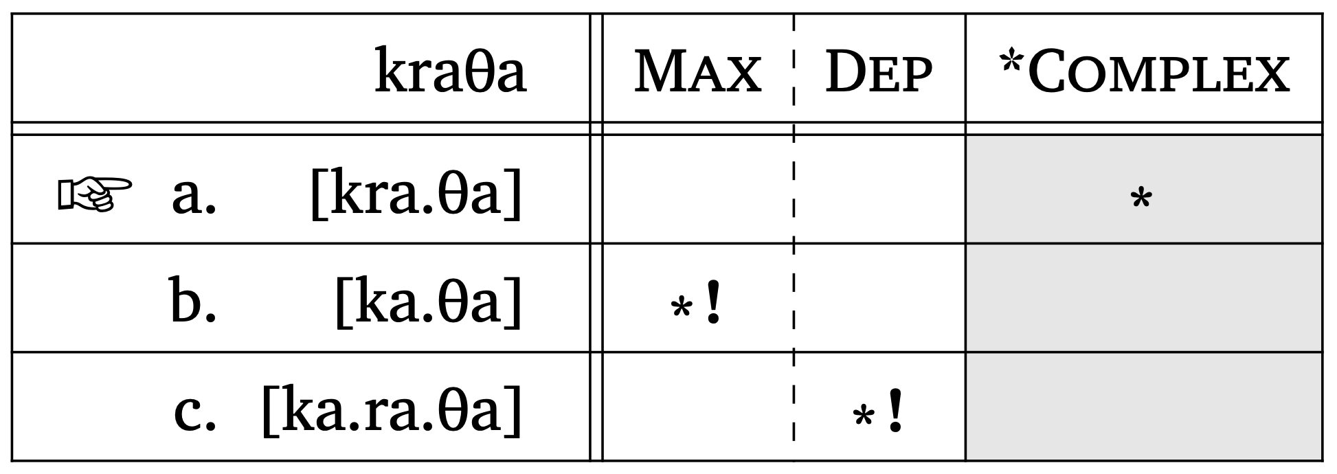
OT tableau
#tableau(
  input: "kraTa",
  candidates: ("kra.Ta", "ka.Ta", "ka.ra.Ta"),
  constraints: ("Max", "Dep", "*Complex"),
  violations: (
    ("", "", "*"),
    ("*!", "", ""),
    ("", "*!", ""),
  ),
  winner: 0,        // position of winning candidate
  dashed-lines: (1,), // note the comma
  shade: true,      // true by default
  letters: true
)
One nice feature of #tableau() is that the function automatically shades cells once a fatal violation is entered (!). Likewise, it adds the “☞” symbol for the winner, whose position is extracted from the winner argument. Candidates can also be labeled with letters (a., b., c., …) by setting letters: true. When letters are used, the ☞ symbol is placed to the left of the winning candidate’s letter.
Additionally, #tableau() supports prosodic structures as candidates.1 You can pass prosodic function calls as content using square brackets, e.g., [#syllable("mat")]. This is the recommended approach because it avoids conflicts with the single quote character, which is also used for stress marking in prosodic notation. Figure 53 shows an example with #word() candidates. When passing content directly, you control the scale via the function’s own scale argument (this is key because prosodic structures as often too large for a tableau). Figure 53 also shows the gloss argument in case more information is needed for the input. This argument requires two strings (orthographic form and translation).
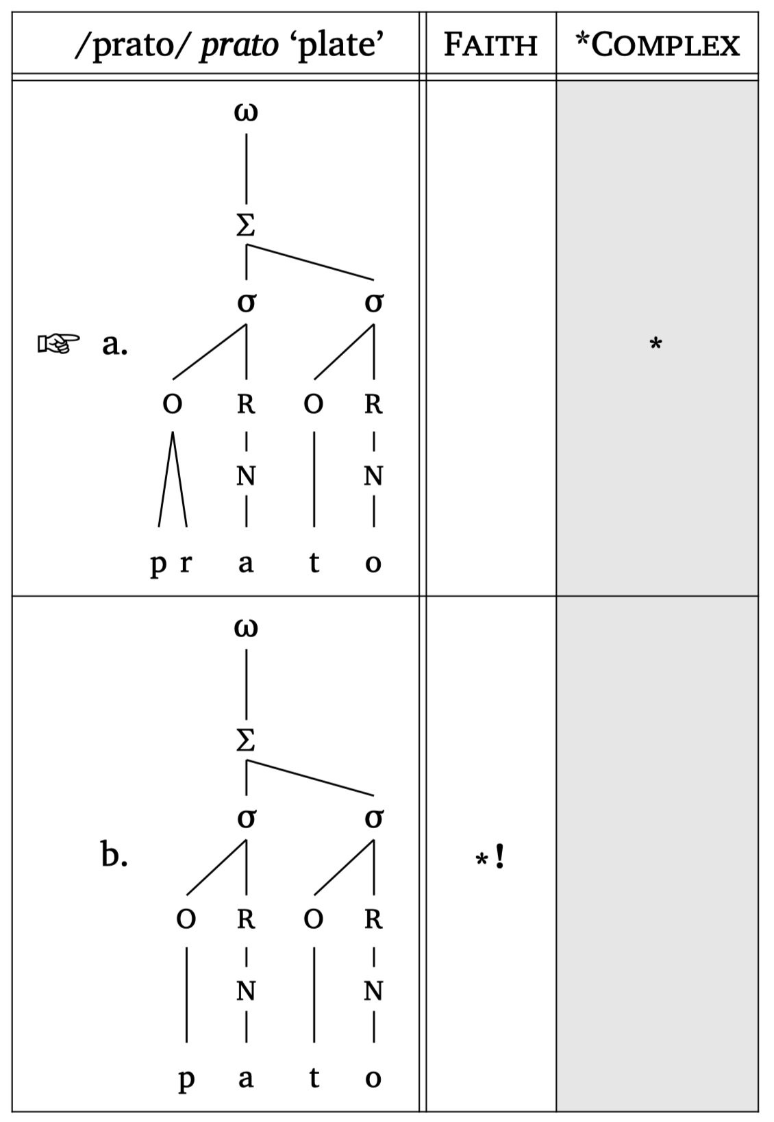
OT tableau + prosody
#tableau(
    input: "prato",
    candidates: (
      [#word("('pra.to)", scale: 0.8)],
      [#word("('pa.to)", scale: 0.8)],
    ),
    constraints: ("Faith", "*Complex"),
    violations: (
      ("", "*!"),
      ("", ""),
    ),
    winner: 0,
    letters: true,
    gloss: ("prato", "plate"),
  )
Hasse diagrams for constraint rankings can be generated with the #hasse() function — see Figure 54 and Figure 55. The function takes tuples with \(n\) elements: a 2-element tuple ("C1", "C2") draws a ranking edge; a 1-element tuple ("C3",) creates a floating constraint. The third element in a tuple controls the “stratum” (vertical position). A fourth element can specify line type: "dashed" or "dotted".
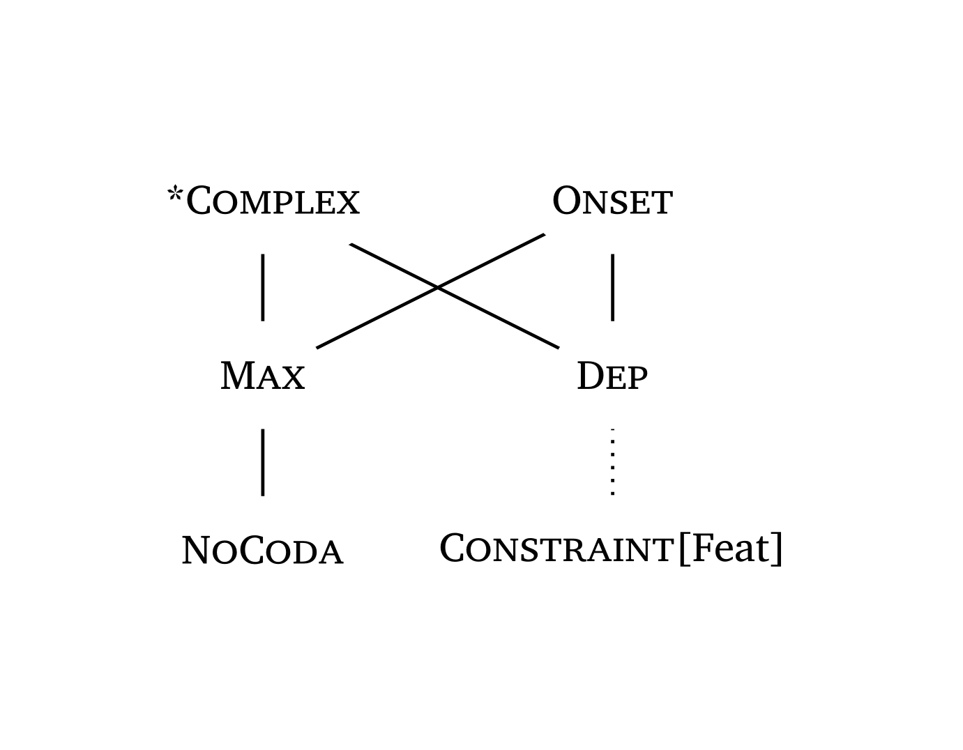
Constraint names are automatically rendered in small caps (except features inside square brackets).
Hasse diagram with dotted lines
#hasse(
(
("*Complex", "Max", 0),
("*Complex", "Dep", 0),
("Onset", "Max", 0),
("Onset", "Dep", 0),
("Max", "NoCoda", 1),
("Dep", "Constraint[Feat]", 1, "dotted"),
),
node-spacing: 3,
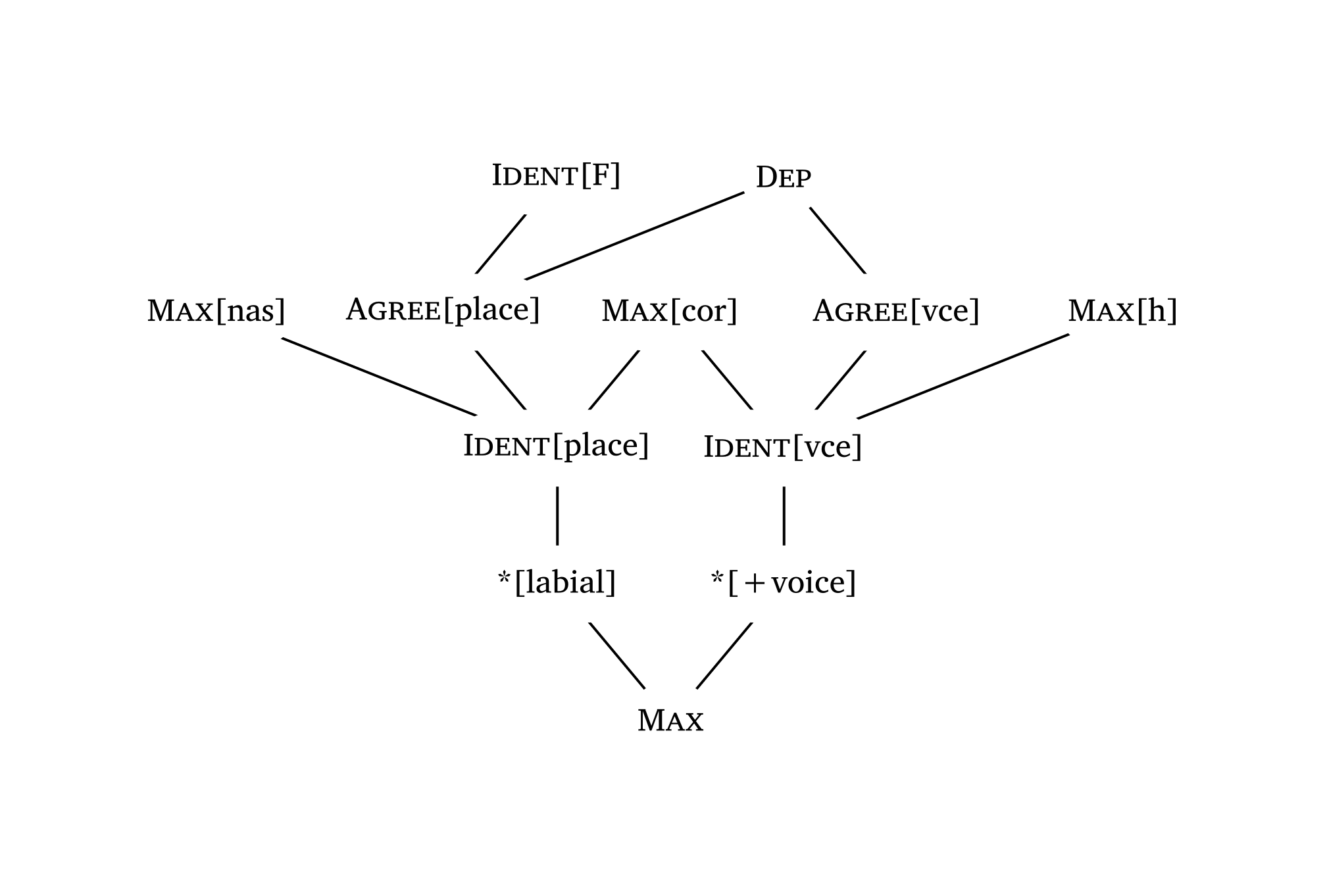
)Complex Hasse diagram
#hasse(
    (
      ("Ident[F]", "Agree[place]", 0),
      ("Dep", "Agree[vce]", 0),
      ("Dep", "Agree[place]", 0),
      ("Max[nas]", "Ident[place]", 1),
      ("Max[cor]", "Ident[place]", 1),
      ("Max[cor]", "Ident[vce]", 1),
      ("Max[h]", "Ident[vce]", 1),
      ("Agree[place]", "Ident[place]", 1),
      ("Agree[vce]", "Ident[vce]", 1),
      ("Ident[place]", "*[labial]", 2),
      ("Ident[vce]", "*[+voice]", 2),
      ("*[labial]", "Max", 3),
      ("*[+voice]", "Max", 3),
    ),
  )
8 Maximum Entropy
The function #maxent() produces a MaxEnt tableau (Goldwater and Johnson 2003; Hayes and Wilson 2008). Given the constraint weights and violations, it automatically calculates \(h_i\), \(e^{-h_i}\), and \(P(y|x)\):
\[P(y|x) = \frac{e^{-\sum_{i=1}^n w_i C_i(y,x)}}{Z(x)}\]
The column \(h_i\) displays the Harmony score (weighted sum of violations); \(e^{-h_i}\) is the unnormalized probability (MaxEnt score); and \(P_i\) is the normalized predicted probability. The function also prints probability bars at the right margin by default (visualize: true, top and bottom in Figure 56). Candidates can be sorted from most to least probable with sort: true (bottom in Figure 56).
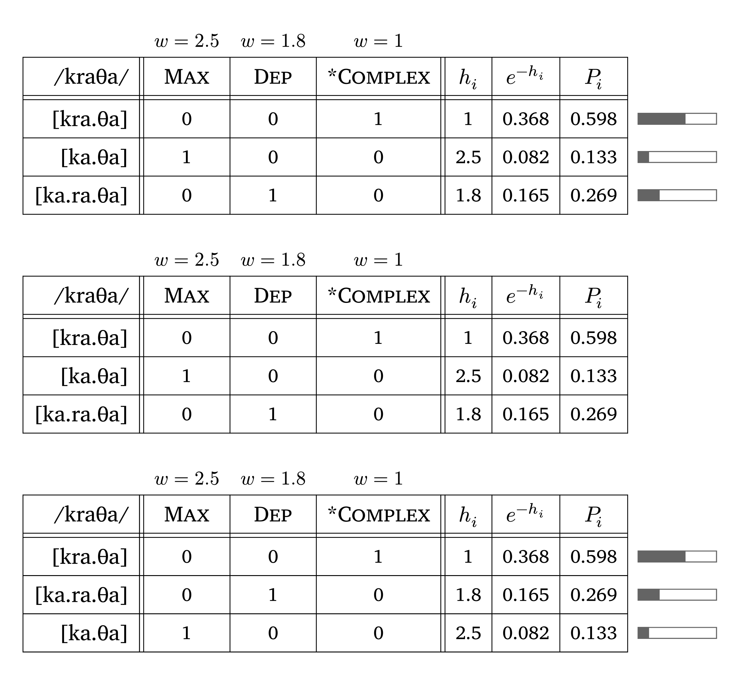
MaxEnt tableau
#maxent(
  input: "kraTa",
  candidates: ("[kra.Ta]", "[ka.Ta]", "[ka.ra.Ta]"),
  constraints: ("Max", "Dep", "*Complex"),
  weights: (2.5, 1.8, 0.5),
  violations: (
    (0, 0, 1),
    (1, 0, 0),
    (0, 1, 0),
  ),
  visualize: true,  // show probability bars (default)
  sort: true        // sort candidates from most to least probable
)phonokit also has functions for Harmonic Grammar (#hg()) and Noisy Harmonic Grammar (#nhg()). These functions share the same syntax as #maxent(), with one important difference: #hg() and #nhg() follow the convention in which violations are negative numbers and the candidate with the highest harmony wins, whereas #maxent() takes positive violation counts. If you reuse a violations array from #maxent(), negate the values first. The #nhg() function derives probabilities by simulating evaluations (default: 1000) given the constraints and violations, and can display the noise column. These functions are based on conventions in Flemming (2021).
9 Numbered examples
The function #ex() creates numbered linguistic examples, accompanied by #subex-label() for labeling each line within an example. Because #ex() is based on tables, the user can customize it with however many columns are needed.
To use this function, add this line after importing the package: #show: ex-rules
Numbered example
// #import "@preview/phonokit:0.5.12": *
// #show: ex-rules  // <- add to your document
// ...
#ex(caption: "A phonology example",
    labels: (<ex-anba>, <ex-anka>),
    columns: (5em, 2em, 5em))[
      - #ipa("/anba/") & #a-r & #ipa("[amba]")
      - #ipa("/anka/") & #a-r & #ipa("[aNka]")
    ] <phon-ex>
ToBI numbered example
#ex(caption: "Some ToBI examples",
    title: [Autosegmental transcription of intonation in English @zsiga2013sounds],
    labels: (<ex-tobi1>, <ex-tobi2>),
    )[
      - You're a we#int("*L")rewolf?#h(1em)#int("H%", line: false)
      - I'm a wer#int("*H")ewolf.#h(1em)#int("L%", line: false)
    ] <tobi-ex>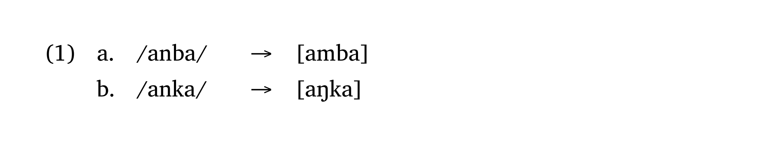
The entire example can be referred to as @phon-ex, and sub-examples can be referred to by their labels (e.g., @ex-anba). Specifying exact column widths (columns: (2em, 2em, 5em, ...)) guarantees perfect alignment across different examples in the document. For ToBI strings, align: left + bottom is essential to ensure letters align with the text baseline rather than the tone annotations.
As of version 0.4.6, a title argument is also available for examples, displayed below the caption number. The caption argument in #ex() is not printed directly — it is there in case you wish to create a table of contents for examples using #outline(target: figure.where(kind: "linguistic-example")).
10 Appendix
10.1 How can I use Typst offline?
While Typst’s own online editor at Typst.app is very useful and practical, most of us prefer to work offline. How can you use Typst offline then?
One of the best IDE options out there is to use VS Code with the extension Tinymist Dreamin and Varner (2024) — the extension is therefore available for Positron, which is the successor to RStudio. Tinymist is also available as a plugin for NeoVim users. All these options work extremely well because Tinymist is great, and I haven’t had any issues thus far: compilation is instantaneous, and bib files also work flawlessly2
If you use Quarto, it is very easy to use phonokit with your qmd files. You need to first declare typst as your format. Then, import the package inside a typst code block and you’re done. Now you’ll be able to use any function you want. Just remember you need the {=typst} suffix every time (which you can automate with a simple snippet in Positron, RStudio, etc.; see here).
    ---
    title: "A Quarto document"
    format: typst
    ---

    ```{=typst}
    #import "@preview/phonokit:0.5.12": *
    ```

    Now you can use any function you want:

    `#syllable("pat"){=typst}`
10.2 Symbols in prosodic representations
As of version 0.3.7, users can decide which symbols are used for prosodic words, feet, syllables, and moras via the symbol argument, which requires an array. The default symbols are Greek letters: \(\omega\), \(\Sigma\), \(\sigma\), \(\mu\).
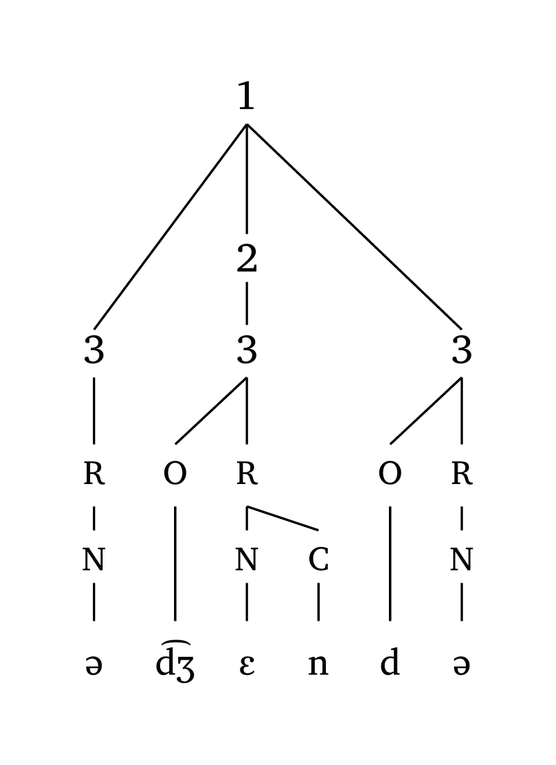
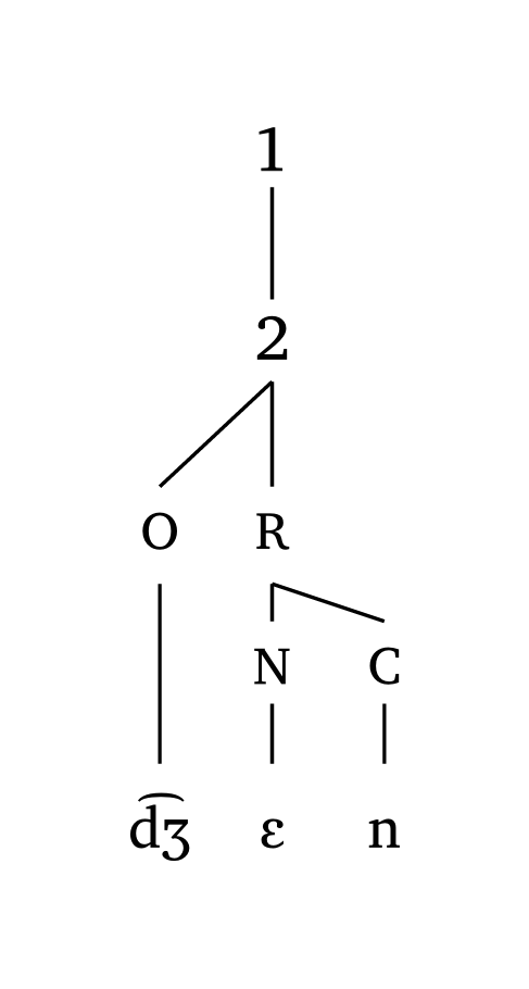
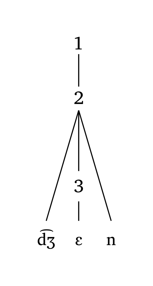
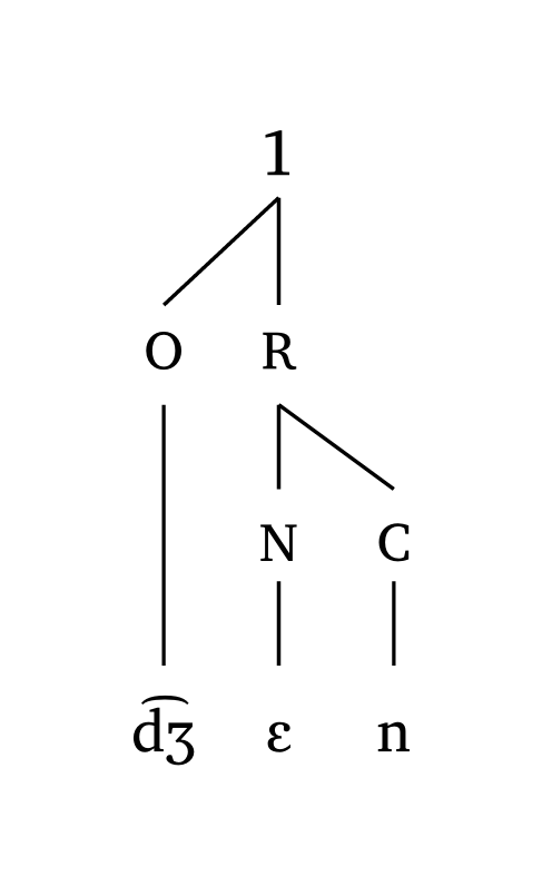
Custom symbols
#word("@.( \\t dZ En).d@", symbol: ("1", "2", "3"))
#foot("\\t dZ En", symbol: ("1", "2"))
#foot-mora("\\t dZ En", symbol: ("1", "2", "3"))
#syllable("\\t dZ En", symbol: ("1",))
10.3 Exporting as images
To use phonokit without adopting Typst as your primary tool, you can export any representation as a PNG. First, create a Typst file with width: auto and height: auto in the page settings:
Typst page setup for export
#import "@preview/phonokit:0.5.12": *
#set page(width: auto, height: auto, margin: 0.5em, fill: none)
// ... your phonokit function here
Then compile from the terminal with:
Compile to PNG (bash)
typst compile file.typ file-{p}.png --ppi 500This generates a PNG file with 500 pixels per inch and transparent background.
10.4 Extras: arrows and Greek letters
The extras.typ module provides convenience symbols.
Arrows:
| Function | Description |
|---|---|
#a-r |
Right arrow |
#a-l |
Left arrow |
#a-u |
Up arrow |
#a-d |
Down arrow |
#a-lr |
Bidirectional arrow |
#a-ud |
Vertical bidirectional arrow |
#a-sr |
Squiggly right arrow |
#a-sl |
Squiggly left arrow |
#a-r-large |
Large right arrow with spacing |
Greek letters (render upright, non-italicized):
| Function | Function | Function |
|---|---|---|
#alpha |
#mu |
#tau |
#beta |
#phi |
#omega |
#gamma |
#pi |
#cap-phi |
#delta |
#sigma |
#cap-sigma |
#lambda |
#cap-omega |
Utilities:
#blank()— underline blank for fill-in exercises or SPE rules; width adjustable:#blank(width: 4em)#extra[...]— wraps content in ⟨angle brackets⟩ for extrametricality
Copyright © Guilherme Duarte Garcia