Maps with R

ggplot2

maps

Author

Guilherme D. Garcia

Published

January 10, 2024

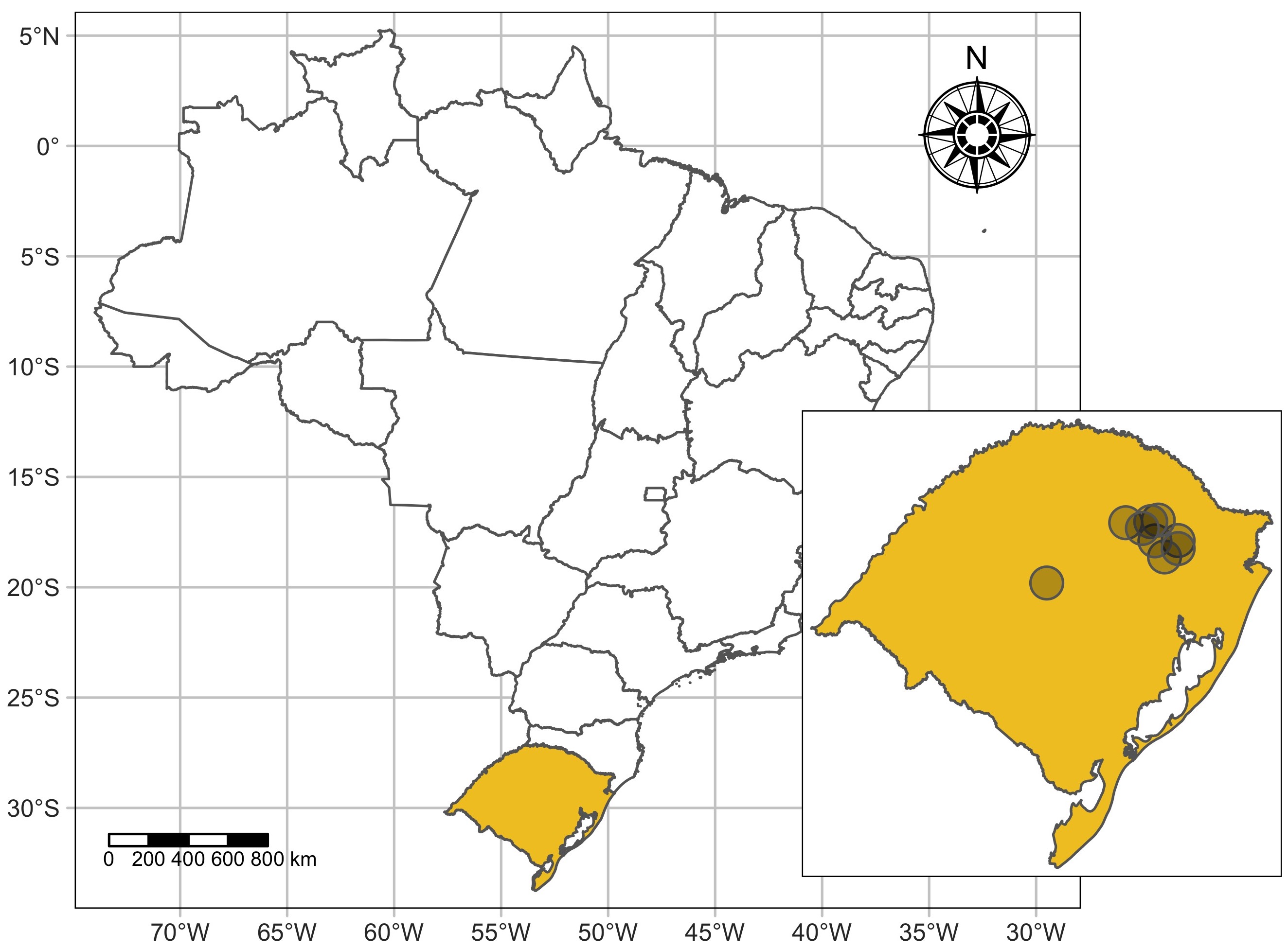
In a recent paper, Natália B. Guzzo and I needed a custom map showing cities in Brazil where Brazilian Veneto has official language status alongside Brazilian Portuguese (Garcia & Guzzo, 2023, p. 117)—the preprint can be accessed here. The result is shown in Figure 1, and the code needed to generate it is detailed below. Essentially, you will need the coordinates for the cities of interest, the map of the country (Brazil) and of the state (Rio Grande do Sul). These can be accomplished with the tidygeocoder, geobr, and tmap packages. Below, we start with a data file that already contains the necessary coordinates, so we won’t be loading leaflet.

Figure 1: The Italian Immigration Area in southern Brazil. Circles represent cities where Brazilian Veneto is an official language.

Loading coordinates

This is a simple table with the relevant cities, their latitude and longitude. Population is also listed but won’t be used here. I’m assuming you already have this. If you don’t, you can use the geo() function from the tidygeocoder extension. For example, geo(address = "Antônio Prado, Brazil", method = "osm") will extract coordinates for the city of Antônio Prado. The extension geobr() also has functions that accomplish the same task.

address	lat	long	pop
Antônio Prado, Rio Grande do Sul	-28.85678	-51.28014	14159
Bento Gonçalves, Rio Grande do Sul	-29.16540	-51.51976	115069
Camargo, Rio Grande do Sul	-28.58657	-52.20315	2524
Caxias do Sul, Rio Grande do Sul	-29.16848	-51.17939	735276
Fagundes Varela, Rio Grande do Sul	-28.88075	-51.69878	2596
Flores da Cunha, Rio Grande do Sul	-29.03013	-51.18333	27135

Designing map

In the code below, we first prepare the data. Next, we create the map for the state in question and, finally, the map for the country.

Code

iia = iia |> 
  separate(address, into = c("city", "state"), sep = ", ") |> 
  filter(state == "Rio Grande do Sul") |> 
  droplevels() |> 
  pull(city)

# Map of the state
states = read_state(year=2019)
rs = geobr::read_state(code_state = "RS")
cities = geobr::read_municipality(year=2019, code_muni = "RS") |> 
  filter(name_muni %in% iia)

# Map of the country
BR = tmap::tm_shape(states) + 
  tmap::tm_graticules(col = "gray80") + 
  tmap::tm_polygons(col = "white") +
  tmap::tm_scale_bar(position = c("left", "bottom"), width = 0.15) +
  tmap::tm_compass(position = c("right", "top"), size = 3, type = "rose") +
  tmap::tm_shape(rs) +
  tmap::tm_polygons(col = "#f1c62a")

RS = tmap::tm_shape(rs) +
  tmap::tm_polygons(col = "#f1c62a") +
  tmap::tm_shape(cities) + 
  tmap::tm_dots(size = 0.8, shape = 21, alpha = 0.25)

The last step is to print the map. This is a bit different from your typical ggplot() figure as we’re placing the state map on top of the country. We’ll use the argument viewport (grid) inside the function print() to accomplish that. To save the map, we’ll use the function tmap_save()—the dimensions in question are exactly the ones we used for Figure 1.

Code

# Printing map
print(BR)
print(RS, vp = viewport(0.8, 0.33, width = 0.5, height = 0.5))


# Saving the figure
tmap_save(tm = BR, filename = "iia.jpeg", 
          insets_tm = RS, 
          insets_vp = viewport(0.8, 0.33, 
                               width = 0.5, 
                               height = 0.5),
          dpi = 500, width = 7, height = 4)

References

Garcia, G. D., & Guzzo, N. B. (2023). A corpus-based approach to map target vowel asymmetry in Brazilian Veneto metaphony. Italian Journal of Linguistics, 35(1), 115–138.