Bayesian estimation in multiple comparisons

Submitted

Author

Affiliations

Guilherme D. Garcia, PhD

Université Laval

CRBLM

Abstract

Traditional regression models typically estimate parameters for a factor F by designating one level as a reference (intercept) and calculating slopes for other levels of F. While this approach often aligns with our research question(s), it limits direct comparisons between all pairs of levels within F and requires additional procedures for generating these comparisons. Moreover, Frequentist methods often rely on corrections (e.g., Bonferroni or Tukey), which can reduce statistical power and inflate uncertainty by mechanically widening confidence intervals. This paper demonstrates how Bayesian hierarchical models provide a robust framework for parameter estimation in the context of multiple comparisons. By leveraging entire posterior distributions, these models produce estimates for all pairwise comparisons without requiring post hoc adjustments. The hierarchical structure, combined with the use of priors, naturally incorporates shrinkage, pulling extreme estimates toward the overall mean. This regularization improves the stability and reliability of estimates, particularly in the presence of sparse or noisy data, and leads to more conservative comparisons. Bayesian models also offer a flexible framework for addressing heteroscedasticity by directly modeling variance structures and incorporating them into the posterior distribution. The result is a coherent approach to exploring differences between levels of F, where parameter estimates reflect the full uncertainty of the data.

Keywords

Bayesian data analysis, multiple comparisons, heteroscedasticity, shrinkage, second language research

1 Introduction

In recent years, studies in second language acquisition have slowly reduced their use of traditional analysis of variance (ANOVAs) accompanied by post-hoc tests, and have instead adopted a wider range of methods, including mixed-effects regression models (e.g., Cunnings, 2012; Plonsky & Oswald, 2017). This is certainly good news, as the field has long relied on a narrow range of statistical methods (e.g., Plonsky, 2014). This change is especially welcome when we consider the misuse of certain techniques. For example, when run on percentages derived from categorical responses, ANOVAs can lead to spurious results (Jaeger, 2008). While ANOVAs are technically a special type of a (linear) regression, their outputs and goals tend to be interpreted slightly differently: ANOVAs are mostly focused on differences between means of levels of a given factor (say, a language group), whereas a typical linear regression is focused on estimating effect sizes for predictor variables, hence the different outputs from both methods. This difference might explain why analyses that employ ANOVAs sometimes carry out multiple comparisons to verify where specific differences may originate in their data. This practice tends to be accompanied by some type of \(p\)-value adjustment to reduce the rate of Type I error.

In this paper, I explore a scenario where an analysis is based on a hierarchical model (also known as mixed-effects model), but where multiple comparisons are needed or desired. More specifically, I show how to generate multiple comparisons using Bayesian estimation from a hierarchical model. Our primary objective in this tutorial is to estimate effect sizes from multiple comparisons, not to reject a null hypothesis per se. That being said, because these two perspectives of statistical analysis often go together in practice, I will refer to hypothesis testing at times. Finally, since one of the best ways to understand and examine estimates from a Bayesian model is to visualize them, this tutorial will have a strong emphasis on data visualization.

Besides the various advantages of Bayesian data analysis in general (Section 3.1), the context of multiple comparisons is especially instructive and beneficial as no correction is needed once we assume non-flat priors (e.g., centered around zero) and a hierarchical structure that leads to shrinkage, naturally yielding more reliable estimates (Section 2). This paper is accompanied by an OSF repository (https://osf.io/37u56/) that contains all the necessary files to reproduce the analysis below. I assume some level of familiarity with the R language (R Core Team, 2024) and with the tidyverse package (Wickham et al., 2019).

2 A typical scenario

The data used in this paper is hypothetical: its structure is adapted from the danish data set presented in Balling & Baayen (2008), which can be found in the languageR package (Baayen, 2009). In their study, the authors designed an auditory lexical decision task with 72 simple words and 232 nonwords. Seven inflectional and nine derivational suffixes were included in the task, each of which was found in 10 words. The response variable, resp, therefore consists of log-transformed reaction times. Noise has been added to a subset of the data in question such that the observations examined in the present paper do not reflect the original data set. Our data set d , shown in Table 1, simulates a common scenario in language acquisition studies, where we are interested in a condition with multiple levels of interest (\(n = 5\))—this is the variable cond in the data. Our data file has 22 participants and 49 items. Furthermore, the number of observations for one of the conditions (c4) has been reduced in order to create an imbalance in the data, as can be seen in Table 2. This situation emulates a small sample size when we consider the number of items per participant—this is certainly not uncommon in second or third language studies (Cabrelli-Amaro et al., 2012; Garcia, 2023).

Table 1: A sample of our data set.

#> # A tibble: 5 × 4
#>   part    item    cond   resp
#>   <fct>   <fct>   <fct> <dbl>
#> 1 part_1  item_1  c5     6.91
#> 2 part_6  item_34 c4     6.74
#> 3 part_19 item_11 c1     6.75
#> 4 part_10 item_36 c1     6.74
#> 5 part_11 item_40 c3     6.76

Table 2: Number of observations per condition (cond), means, variances, and standard deviations of responses (resp).

#> # A tibble: 5 × 5
#>   cond      n  Mean    Var    SD
#>   <fct> <int> <dbl>  <dbl> <dbl>
#> 1 c1      209  6.81 0.0402 0.200
#> 2 c2      215  6.76 0.0460 0.214
#> 3 c3      189  6.86 0.0339 0.184
#> 4 c4       50  6.85 0.0357 0.189
#> 5 c5      213  6.75 0.0253 0.159

Our data set has four (self-explanatory) variables: part, item, cond and resp. Ultimately, we want to verify if participants’ (part) responses (resp) are affected by our five conditions (cond) taking into account the expected variation found across participants (part) and items (item). The five hypothetical conditions in the data set are c1 to c5. We will start our analysis by visually exploring the patterns in the data, shown in Fig. 1.

Figure 1: Overall patterns in the data: box plots and associated means (orange dots) and standard errors (not visible).

Our response variable is continuous and approximately Gaussian (otherwise we should avoid box plots), so we can rely on our familiar parameters (e.g., our means for each condition) for statistical inference. Typically, we would now run a hierarchical linear regression where cond is our predictor variable using the lmer() function from the lme4 package (Bates & Maechler, 2009). In Code block 1, such a model is run with by-participant and by-item random intercepts, fit1, the maximally-converging model given the data.

Code block 1: Hierarchical linear regression.

# Packages used to run code below:
library(lme4)
library(lmerTest) # To display p-values in output
library(emmeans)  # For multiple comparisons

# Hierarchical model using lme4 package:
fit1 = lmer(resp ~ cond + (1 | part) + (1 | item),
            data = d)

# Printing only our fixed effects:
summary(fit1)$coefficients |> round(2)
#>             Estimate Std. Error    df t value Pr(>|t|)
#> (Intercept)     6.81       0.03 54.56  223.61     0.00
#> condc2         -0.06       0.04 37.10   -1.57     0.12
#> condc3          0.05       0.04 37.27    1.35     0.18
#> condc4          0.02       0.04 65.24    0.45     0.65
#> condc5         -0.07       0.04 37.16   -1.87     0.07

As is typical in regression models with a categorical predictor variable, we can see that condc1 is automatically used as our reference level (intercept, \(\hat\beta_0\)), to which all other levels of cond are compared.

Thanks to packages such as lme4 and emmeans, a few lines of code are sufficient to run hierarchical regression models and generate multiple comparisons deriving from them—this is shown in Code block 2 and Code block 3. If we were merely interested in null hypothesis significance testing, using the Tukey-adjusted comparisons in Code block 2, we would identify two comparisons (c2-c3 and c3-c5) as statistically significant (\(p < 0.05\)).

Code block 2: Tukey-adjusted pairwise comparisons of group means using the emmeans package.

# Multiple comparisons with emmeans package:
emmeans(fit1, pairwise ~ cond, adjust = "tukey")$contrasts
#>  contrast estimate     SE   df t.ratio p.value
#>  c1 - c2    0.0555 0.0353 38.1   1.571  0.5243
#>  c1 - c3   -0.0492 0.0363 38.3  -1.354  0.6598
#>  c1 - c4   -0.0186 0.0413 66.9  -0.449  0.9914
#>  c1 - c5    0.0660 0.0353 38.2   1.869  0.3508
#>  c2 - c3   -0.1047 0.0363 38.0  -2.886  0.0473
#>  c2 - c4   -0.0740 0.0413 66.6  -1.793  0.3861
#>  c2 - c5    0.0105 0.0353 37.9   0.299  0.9982
#>  c3 - c4    0.0306 0.0421 65.2   0.726  0.9496
#>  c3 - c5    0.1152 0.0363 38.1   3.176  0.0233
#>  c4 - c5    0.0846 0.0413 66.7   2.048  0.2550
#> 
#> Degrees-of-freedom method: kenward-roger 
#> P value adjustment: tukey method for comparing a family of 5 estimates

Code block 3: Bonferroni-adjusted pairwise comparisons of group means using the emmeans package.

emmeans(fit1, pairwise ~ cond, adjust = "bonferroni")$contrasts
#>  contrast estimate     SE   df t.ratio p.value
#>  c1 - c2    0.0555 0.0353 38.1   1.571  1.0000
#>  c1 - c3   -0.0492 0.0363 38.3  -1.354  1.0000
#>  c1 - c4   -0.0186 0.0413 66.9  -0.449  1.0000
#>  c1 - c5    0.0660 0.0353 38.2   1.869  0.6927
#>  c2 - c3   -0.1047 0.0363 38.0  -2.886  0.0639
#>  c2 - c4   -0.0740 0.0413 66.6  -1.793  0.7747
#>  c2 - c5    0.0105 0.0353 37.9   0.299  1.0000
#>  c3 - c4    0.0306 0.0421 65.2   0.726  1.0000
#>  c3 - c5    0.1152 0.0363 38.1   3.176  0.0296
#>  c4 - c5    0.0846 0.0413 66.7   2.048  0.4450
#> 
#> Degrees-of-freedom method: kenward-roger 
#> P value adjustment: bonferroni method for 10 tests

The scenario above is common insofar as many studies in second language research involve a continuous response variable and a factor for which multiple comparisons can be useful. Nevertheless, the statistical methods employed in such situations often vary in the literature, and sometimes ignore the intrinsic hierarchical structure of the data altogether (e.g., linear regression models without random effects). Before proceeding, it is worth discussing why a hierarchical model is not only necessary given our data, but also why it is advantageous in the context of multiple comparisons, the topic of the present paper.

2.1 Why hierarchical models?

Hierarchical models are preferred when dealing with data that has inherent grouping structures, such as repeated measures across subjects or items. Unlike simpler models that ignore or simplify within-group variability, hierarchical models incorporate both fixed effects (e.g., the variable cond in our data) and random effects (e.g., part and item in our data). In the context of data with repeated observations per subject and item, in which the independence assumption is violated, hierarchical models can account for these sources of variability, allowing for more accurate estimates that reflect the true complexity of the data. By including random intercepts or slopes, hierarchical models can capture subject- or item-specific influences, which results in a more nuanced understanding of the effects being studied.

One important aspect of hierarchical models involves a process called shrinkage (also known as partial pooling). Shrinkage adjusts the estimates for random effects by pulling extreme estimates closer to the group mean. This regularization reduces the impact of outliers or overly variable estimates, leading to more stable and conservative results. As will be seen below, shrinkage can also affect fixed effects estimates, a key point in the analysis that follows.

Before hierarchical models became mainstream in second language studies, a popular method of analysis involved running separate ANOVAs on data aggregated by subject and by item. There are, of course, negative consequences of such a method. First, two analyses are needed a priori, one for subject-aggregated data, one for item-aggregated data. As a result, participant- and item-level predictors cannot be included in the same analysis. Second, missing items in one or more condition levels must be removed. Third, ANOVAs do not typically focus on effect sizes, which in turn requires a separate method to quantify the magnitude of effects (e.g., \(\eta^2\)). We will not discuss ANOVAs in this paper, but one of the linear models we will discuss next (LM) is equivalent to an ANOVA run on participant-aggregated data.

Examine Fig. 2, where three different models for our data are compared. Along the \(x\)-axis, LM represents a simple linear regression run over the aggregated mean response by participant for each condition. LM+B represents the same model with a Bonferroni correction, which affects the confidence interval of each estimate (but notice that standard errors are not affected). Finally, HLM shows the estimates from the hierarchical model from Code block 2. Notice how the estimate for c4 (highlighted in the figure) is substantially closer to the grand mean, i.e., it has shrunk. In addition, the confidence intervals shown under HLM are wider than the intervals under LM.¹ Given these two characteristics of the HLM in question, multiple comparisons stemming from such a model are more reliable and generally more conservative than those performed from LM or LM+B—this will also be clear when we examine our model figure later. It is also worth reiterating that HLM includes both by-participant and by-item random intercepts in the same analysis, and is therefore objectively more complex and more comprehensive than the other two models. The reader can find a similar scenario and a more detailed discussion in Gelman et al. (2012).

Figure 2: Estimate comparison across three models (\(x\)-axis). Standard errors (horizontal lines) and 95% confidence intervals (vertical lines) are also shown for each estimate. Dashed line represents the average across all conditions (panels on top).

Shrinkage is not always visible in the estimates of our fixed effects, since its effect is more directly observable in our random effects. The reason why we do see shrinkage in our estimate for c4 here is because our data is imbalanced: condition c4 has only 50 observations (cf. \(n=\) 189–215 for the other conditions). This represents a situation that we often encounter, where a particular group of interest is imbalanced and may have too much influence on the estimates of our models. Our hierarchical model here mitigates the problem by pulling the estimate of c4 towards the grand mean, since it does not have enough empirical evidence (i.e., observations) to grant the estimate provided by LM and LM+B.

In general, then, hierarchical models allow for more reliable confidence intervals even without corrections such as Bonferroni, a desirable characteristic, given that such corrections typically reduce statistical power and tend to modify only confidence intervals (or \(p\)-values), keeping estimates stationary. Hierarchical models also reduce the issue of multiple comparisons, since point estimates can be shifted (shrinkage), as demonstrated above—see Gelman & Tuerlinckx (2000), Gelman et al. (2012) and Kruschke (2015, pp. 567–568). And because multiple comparisons are derived from the estimates of each level being compared, more reliable estimates in our models lead to more reliable comparisons from said models.

In the sections that follow, we will reproduce the analysis in Code block 1 using a Bayesian approach. In doing so, we will also discuss fundamental differences between Frequentist and Bayesian statistics, and how favoring the latter can offer intuitive insight on the estimation of parameters, especially when it comes to multiple comparisons.

3 Methods

In this section, I provide a brief introduction to Bayesian data analysis and review the packages that will be used in Section 4.

3.1 A brief review of Bayesian data analysis

This section will focus on the minimum amount of information needed on Bayesian data analysis for the remainder of this paper. With such an immense topic, anything more than the basics would be unrealistic given the scope of the present paper. A user-friendly introduction to the topic is provided in Kruschke & Liddell (2018), Garcia (2021, ch. 10) and Garcia (2023). Comprehensive introductions to Bayesian data analysis are provided in McElreath (2020) and Kruschke (2015).

A typical statistical test or model generates the probability of observing data that is at least as extreme as the data we have given a particular statistic (e.g., \(\hat\beta\)) under the null hypothesis. This is the definition of p-values, a concept inherently tied to the notion of Type I error and the corrections often applied when conducting multiple comparisons. In contrast, Bayesian approaches do not use \(p\)-values, and therefore do not have a family-wise error rate in the traditional Frequentist sense. However, this does not eliminate the possibility of spurious results or false positives, which can occur regardless of the statistical framework employed. In Frequentist data analysis, then, we are after \(P(data|\pi)\), where \(\pi\) is any given statistic of interest. In this framework, we think of “probability” as the frequency of an event in a large sample—hence the name Frequentist and the importance of larger samples.

In a Bayesian framework, we generate the probability of a parameter given the data, i.e., the opposite of what we get in a Frequentist framework. In other words, we are given \(P(\pi|data)\), which allows us to estimate the probability of a hypothesis. The essence of Bayesian data analysis comes from Bayes’ theorem (Bayes, 1763; also see McGrayne, 2011), shown in Equation 1. The theorem states that the posterior, \(P(\pi|data)\), is equal to the likelihood of the data, \(P(data|\pi)\), times the prior \(P(\pi)\), divided by the marginal likelihood of the data, \(P(data)\).

\[P(\pi|{data}) = \frac{P({data}|\pi) \times P(\pi)}{P({data})} \tag{1}\]

One crucial component in Bayes’ theorem is the prior, which allows us to incorporate our expectations into the model. These expectations are informed by the literature: if we know about a particular phenomenon, it is just natural that this knowledge should be included in a model. Not only is this aligned with the accumulation of knowledge assumed in science (e.g., Brand et al., 2019), but it also bridges a common gap between our theoretical assumptions and our data analysis, which typically ignores any prior knowledge that we may have on the object being analyzed. A third advantage of priors is the fact that they can cause shrinkage even in non-hierarchical models. As discussed above, shrinkage is an advantage insofar as it improves the reliability of our estimates by decreasing the influence of noise in the data, pulling extreme values towards the mean.

Even though the notion of priors is intuitive, some may argue that priors can bias our model. This can be true: if we force our priors to be where we want them to be with a high degree of certainty, the posterior distribution will be strongly biased towards our priors. This, however, is not how priors are supposed to work—see Gelman (2008) on common objections to Bayesian data analysis and Gelman & Hennig (2017) on the notions of objectivity and subjectivity in statistics. Priors must be informed by the literature and by previous experiments. Furthermore, our certainty surrounding prior distributions must reflect the state of knowledge surrounding the object being examined. If we have over one hundred studies showing that an effect size is between 1.2 and 1.4, we could certainly assume a prior distribution centered around 1.3. Considering a Gaussian prior distribution, we could even set its standard deviation to a low number to incorporate the high degree of precision in the literature in this scenario.

Bayesian models estimate effects by sampling from the posterior distribution by using a wide range of algorithms, not by solving the theorem above analytically (which is computationally impossible even for relatively simple models). Think of this sampling as a “random walk” in the parameter space²—this is indeed the typical metaphor employed for Markov-Chain Monte Carlo methods, which are commonly associated with posterior sampling. Suppose we are interested in the difference in means between two groups. Our model will consider a multitude of possible values for this difference. Each value will yield a probability: “take value 0.7 and calculate the probability of observing this value given the data being modelled”. After enough values are considered (i.e., iterations), the sampling algorithm will have visited values that are more likely (given the data) more frequently. This clustering gives us our posterior distribution for the parameter in question, i.e., the difference between the two groups. In reality, we will use a language called Stan (Carpenter et al., 2017), which employs an algorithm called Hamiltonian Monte Carlo (HMC). A “random walk” is not the best way to describe HMC, but the idea is still valid for our purposes here. Fig. 3, from Garcia (2021, p. 220), illustrates the end of a random walk for two parameters in a regression model, \(\hat\beta_0\) and \(\hat\beta\), which results in a joint posterior distribution where the most visited values for both parameters in question are at the peak of the distribution.

Figure 3: Illustrative example of the joint posterior distribution of two parameters in a regression model

You may be wondering how we can know that the model has correctly converged onto the right parameter space, i.e., the right parameter values given the data. Our algorithms use multiple chains to explore said space. If all chains (typically four) converge by the end of the sampling, we know the model has converged. We can check this convergence in different ways. For example, we could visually inspect the chains to see if they have clustered in a particular region.

In this paper, we will use an intuitive R package to run our models, so you do not have to worry about learning the specifics of Stan to be able to run and interpret Bayesian models. Interestingly, on the surface, our models will look quite similar to their Frequentist counterparts. Deep down, however, they work in very different ways, and their interpretation is much more intuitive than what we are used to in Frequentist models. First, p-values no longer exist. Second, effects are not given as point-estimates. Rather, they are entire probability distributions of credible effects given the data, which substantially affects how we interpret and visualize our models’ results, as we will see later.

3.1.1 Hypothesis testing and parameter estimation

As previously mentioned, our main goal here is to estimate effect sizes in multiple comparisons. To do that, we will focus on credible intervals, which are illustrated and discussed in the Bayesian model examined in Section 4 below. One specific type of credible interval we can use is the highest density interval (HDI), which gives us a particular percentage of the most probable parameter values given the data. Simply put, values inside such an interval are more likely than values outside of it—this is a much more intuitive interpretation than Frequentist confidence intervals. When we focus our analysis on parameter estimation, we are merely asking the question: what are the most likely values for our parameters given the data (and our priors)?

Credible intervals allow us to answer the question above, but they should not be used as our main metric to confirm or reject the existence of an effect, since the null model (one that does not include the variable(s) of interest) is not under evaluation (see, e.g., Veríssimo (2024)). This brings us to the secondary dimension of our analysis here, namely, the notion of hypothesis testing. A Bayesian model that includes cond as a predictor describes an alternative hypothesis according to which we believe that the variable cond has an effect. As we run such a model and inspect its credible intervals, nothing is directly revealed about the null model, i.e., the model without cond as a predictor, since that model is not being evaluated. Note that this is different from what we can conclude from confidence intervals in Frequentist models, where, if zero is not contained inside an interval, we can indeed reject the null hypothesis.

The topic of hypothesis testing in Bayesian statistics often involves the use of Bayes Factors. A Bayes Factor is a ratio used to quantify the evidence for a particular hypothesis relative to another hypothesis (or multiple hypotheses). In our scenario, we could run a null model (bFitNull; intercept-only) and calculate the Bayes Factor of a model containing cond (bFit1) relative to said null model. This is shown in Equation 2.

\[ BF_{10} = \frac{P(data|H_1)}{P(data|H_0)} \tag{2}\]

A Bayes Factor greater than 1 indicates evidence in favor of bFit1 (our alternative model). A Bayes Factor less than 1 indicates evidence in favor of bFitNull (our null model). If we reach a Bayes Factor of 1, we have no evidence to decide which model/hypothesis is more likely. While this paper does not use Bayes Factors, it is certainly an important topic to those who wish to test hypotheses in a Bayesian framework. The reader will benefit from the appendix provided in Kruschke (2013), where the author discusses the shortcomings of Bayes Factors (p. 602), which can at times hide crucial information about parameter uncertainty. A detailed and user-friendly discussion on estimation and hypothesis testing is also provided in Veríssimo (2024, pp. 12–15).

Another method of exploring hypothesis testing in Bayesian models involves the definition of a region of practical equivalence (ROPE). In a nutshell, we calculate an area around zero, and if most or all of our HDI of interest falls within that area, we conclude that we have sufficient evidence for a null effect (i.e., we reject the alternative and accept the null). Conversely, if the entire HDI falls outside the ROPE, we reject the null. In the remainder of this tutorial, we will make use of ROPEs as we interpret the results of our estimates and the multiple comparisons derived from them. ROPEs will be favored because they can be easily generated and incorporated into our figure as we estimate parameters and the uncertainty around them, our primary goal here as we approach multiple comparisons. By including ROPEs in our analysis, we will also have a small component of hypothesis testing, i.e., we will potentially be able to accept/reject a null effect if that scenario arises.

Next, we will see the notions discussed above in action, as we run and analyze our model. In summary, we will use highest density intervals (HDI) to estimate the most credible values of our parameters (our primary goal), and we will also use a region of practical equivalence (ROPE) to quantify the evidence for the effect of cond (our secondary goal).

3.2 Data and packages

In Code block 4, you will find the data file as well as the necessary packages to reproduce the analysis in the paper. You will all the packages below before proceeding. The package brms (Bürkner, 2016) allows us to run Bayesian models by using the familiar syntax from functions such as lm() and glm(). Finally, tidybayes (Kay, 2020) and bayestestR (Makowski et al., 2019) will help us work with posterior samples.

Code block 4: Packages used in the paper.

# In addition to the packages already loaded:
library(tidyverse)
library(brms)
library(tidybayes)
library(bayestestR)

4 Analysis

4.1 Statistical model

In this subsection, we will run our hierarchical Bayesian model, which will have a single fixed predictor (cond). I will assume that you have never run a Bayesian model or used the brms package. While specific details of our models are outside the scope of this paper, I will attempt to provide all the necessary information to reproduce and apply these methods to your own data. In the next subsection, we will work on our multiple comparisons based on the model bFit1 that we run and discuss below.

In Code block 5, we define our model as resp ~ cond using the same familiar syntax from the lm() function. Notice that this is the most complex model thus far, as it includes random slopes for cond by participant—this model specification yields a singular fit using a Frequentist approach with lmer(). Because we are running a linear regression, we assume that the response variable is normally distributed, hence family = gaussian() in the code. We could also use another family value if we wanted to better accommodate outliers. For example, we could specify family = student(), which would assume a student \(t\) distribution for our response variable resp. This can be useful in situations where we have smaller sample sizes (higher uncertainty) and/or potential outliers.

By default, our model will use four chains to sample from the posterior. To speed up the process, we can use four processing cores. The argument save_pars is necessary if the reader wishes to calculate the Bayes Factor later on using the bayes_factor() function in brms. If that is the case, a null model is also needed: that is why bFitNull is also present in the code. The reader can run both models and subsequently run bayes_factor(bFit1, bFitNull) to confirm that the Bayes Factor will favor the alternative hypothesis, i.e., that cond indeed has an effect on resp—the line is commented out in Code block 5 because we will not explore those results, as mentioned above. Finally, we set our priors (see below) and save the model (optionally) to have access to the compiled Stan code later. While this last step is not necessary, if you want to better understand the specifics of our model, it is useful to examine the raw Stan code later on.

Code block 5: A simple hierarchical linear regression using brms.

# Our model assumes that cond has an effect:
bFit1 = brm(resp ~ cond + (1 + cond | part) + (1 | item),
            data = d, 
            family = gaussian(), 
            cores = 4, 
            prior = priors1,
            save_pars = save_pars(all = TRUE),
            save_model = "bFit1.stan")

# What a null model looks like:
bFitNull = brm(resp ~ 1 + (1 | part) + (1 | item),
               data = d, 
               family = gaussian(), 
               cores = 4, 
               iter = 4000,
               prior = priorsNull,
               save_pars = save_pars(all = TRUE),
               save_model = "bFitNull.stan")

# To generate our Bayes Factor:
# bayes_factor(bFit1, bFitNull)

The model in question, bFit1, will not run until we create the variable priors1 referred to in the code. First, it should be clarified that we do not need to specify priors ourselves: brm() will use its own set of default priors if we do not provide ours. Here, however, we will assume some mildly informative priors. The default priors used by brm() will often be flat, which means the model starts by assuming that values are equally likely. This, however, is neither realistic nor ideal: given the data at hand, we know that no responses are lower than 4 or higher than 8 given Fig. 1.³ We also know that extreme reaction times are unlikely in the literature of lexical decision tasks. Importantly, we know that not all values for our condition levels are equally likely. Imagine that we were estimating the height of a given person. A height of seven meters is clearly impossible, and our model should not start by assuming that such an extraordinary height is just as likely as, say, 1.75 meter. Likewise, a reaction time of 6 (approximately 400ms) of much more likely than a reaction time of 10 (approximately 22,000ms) in such tasks, and reaction times under 2 (approximately 100ms) are considered to be unreliable (Luce, 1991; Whelan, 2008).

Code block 6: How to access and set our own priors in brms.

# See output of get_prior() in Code block 6 below
get_prior(resp ~ cond,
          data = d, cores = 4, family = gaussian())

priors1 = c(set_prior(class = "Intercept", 
                      prior = "normal(7, 1)"),
            set_prior(class = "b", # all slopes
                      prior = "normal(0, 1)"))

# Priors for the null model bFitNull:
priorsNull = c(set_prior(class = "Intercept", 
                         prior = "normal(7, 1)"))

Code block 7: The structure of priors in brms.

# A simplified output of get_prior():
get_prior(resp ~ cond,
          data = d, cores = 4, 
          family = gaussian()) |> 
  select(prior, class, coef, source)
#>                   prior     class   coef  source
#>                  (flat)         b        default
#>                  (flat)         b condc2 default
#>                  (flat)         b condc3 default
#>                  (flat)         b condc4 default
#>                  (flat)         b condc5 default
#>  student_t(3, 6.8, 2.5) Intercept        default
#>    student_t(3, 0, 2.5)     sigma        default

In Code block 6, we first use the function get_prior() to inspect the priors assumed by the model (default priors). The reader can inspect the output of get_prior() in Code block 7. Note that we are feeding get_prior() with the non-hierarchical version of the model to simplify our analysis here, but you could certainly extract and modify priors on the mixed effects as well. We then set our own priors with the function set_prior(). Here, we are assuming that all of slopes (c2 to c5) follow a Gaussian (normal) distribution centered around zero with a standard deviation of 1: \(\mathcal{N}(\mu = 0, \sigma = 1)\). Thus, the priors in question contain no directional bias, and they also introduce a relatively high degree of uncertainty, given the standard deviation we assume for each distribution. For comparison, in our actual data, the standard deviation of our response variable resp ranges from \(0.16\) to \(0.21\) for all five conditions cond, as can be verified in Table 2.⁴ These priors tell the model that absurd values are simply not plausible. Finally, our intercept (\(\hat\beta_0\)) is assumed to have a mean of 7 (which approximates the observed mean of c1 already visualized).

In summary, we are telling our model that there should be no differences between the conditions, and we are constraining the range of potential differences by saying that values near zero are more likely than values far away from zero. This starting point is very distinct from assuming flat priors. We are merely telling the model that certain values are much more likely than others, and we are being conservative by assuming priors centered at zero with relatively wide distributions.

Since we have now defined our priors, we can finally run our model. Running a Bayesian model takes much longer than running an equivalent Frequentist model. For that reason, it is a good idea to save the model for later use: save(bFit1, file = "bFit1.RData") will save the model in RData format. You can later read it by using load("bFit1.RData"). Importantly, we can save however many objects in a single RData file. The Population-level effects of our model, bFit1, are shown in Code block 8—the reader should run bFit1 to explore the entire output of the model.

Code block 8: Model results (only population-level).

summary(bFit1)$fixed |> round(2)
#>           Estimate Est.Error l-95% CI u-95% CI Rhat Bulk_ESS Tail_ESS
#> Intercept     6.81      0.03     6.75     6.88    1   891.03  1753.07
#> condc2       -0.06      0.04    -0.13     0.02    1  1436.42  2309.61
#> condc3        0.05      0.04    -0.03     0.12    1  1431.52  2217.36
#> condc4        0.03      0.05    -0.07     0.12    1  1710.44  2504.72
#> condc5       -0.07      0.04    -0.14     0.00    1  1360.37  2387.45

In the column Estimate, we can see the mean estimate for each condition (recall that each estimate is in fact an entire posterior distribution). We also see the error for each estimate (i.e., the standard deviation of the posterior distribution),⁵ and the two-sided 95% credible intervals (l-95% CrI and u-95% CrI) based on quantiles Bürkner (2017, p. 11). For symmetrical posterior distributions (e.g., Gaussian distributions), this interval coincides with the Highest Density Interval (HDI)—to calculate the exact 95% HDI of a fit, we can use the hdi() function from the bayestestR package. Following Kruschke (2015, p. 342), I will favor HDIs over CrIs in the present paper, as they offer a more intuitive interpretation when we consider skewed distributions—a type of distribution we will not examine in this paper.

Next, we see Rhat (\(\hat{R}\) should be \(< 1.01\)),⁶ which tells us that the model has converged. Finally, we see two columns showing us the effective sample size (ESS) of our posterior samples: the bulk ESS corresponds to the main body of the posterior distribution, while the tail ESS corresponds to the tails (i.e., more extreme values) in the posterior distribution. By default, each of the four chains draws 2,000 samples from the posterior. However, we use a warmup of 1,000 samples. As a result, only 1,000 samples from each chain are actually used here, totaling 4,000 samples. Of these 4,000, however, some “steps” in our random walk will be correlated with one another, which reduces the amount of information they provide about the parameter space. Therefore, we should prioritize uncorrelated steps, which results in a proper subset of the 4,000 steps in question. That’s why all the numbers in both ESS columns are less than 4,000. There is no universal rule of thumb as to how large the ESS should be (higher is always better, of course), but 100 samples per chain is a common recommendation. If the ESS is lower than 400, we could increase the number of steps by adding iter = 4000, for example, which would give us 3,000 post-warmup steps for each chain.⁷ We can also change the number of warmup steps in the model, allowing it to “settle” in more informative regions of parameter values before extracting the samples we will actually use.

The reader will notice that the estimates in our Bayesian model are not very different from the estimates in our Frequentist model, run in Code block 1. This makes sense, since our priors are only mildly informative. Ultimately, the posterior distribution in our model is (mostly) driven by the patterns in the data. In a more realistic application, we would attempt to set more precise priors given what we know from the literature on the topic of interest.

While tables can be useful to inspect the results from our model, figures are often a better option as they show the actual posterior distribution for each parameter in our model. In this paper, I will employ a specific type of figure, shown in Fig. 4. The figure contains different pieces of information, some of which are standard in Bayesian models. First, note that a dashed line marks zero. Around that line, we find the ROPE. Now, we can assess the posterior distribution and the HDI of each parameter (our primary goal) as well as their location relative to the ROPE (our secondary goal). As usual, all conditions in the figure must be interpreted relative to c1 (our intercept; not shown). The central portion of each distribution represents the most likely values given the data. It is important to reiterate that the HDIs in the figure are a summary statistic from actual probability distributions, unlike Frequentist confidence intervals. As such, values at the tails of the HDIs are less likely than values at the center of the HDIs. The figure therefore gives us a comprehensive view of effect sizes and parameter estimation.

Next, we can move to our secondary goal. The reader will notice that all of our posterior distributions include zero in their 95% HDI. Logically, this means that every posterior in Fig. 4 is at least in part within the ROPE. Simply put, zero is a credible parameter value representing the difference between each of c2-c5 and c1. That being said, we should also observe the how much of each distribution is within the ROPE. For example, as we compare the distributions of c5 and c4, we can see that a null effect is more likely for c4 than for c5, even though we cannot accept any null effect for the slopes in question, given that no HDI is entirely within the ROPE.

Figure 4: Posterior distributions from hierarchical model with associated 95% HDIs. Region of practical equivalence is represented by shaded area around zero.

4.2 Multiple comparisons

In this section, we will use our hierarchical model bFit1 to extract all the multiple comparisons we wish. There are at least two ways of accomplishing this task. The easy (automatic) way involves a function called hypothesis() from brms. While this function does provide us with estimates on any contrast of interest, its main application is in hypothesis testing, i.e., our secondary goal here—see example in Veríssimo (2024) (p. 14). Still, because at times this is what is needed, and because it is an easy approach to implement, we will start by exploring the function in question in Section 4.2.1. Then, in Section 4.2.2, we will work our way through a more manual approach that will focus on our primary goal here, namely, parameter estimation.

4.2.1 Comparisons via hypothesis testing

Given the levels of our factor cond, we will begin by defining a null hypothesis, represented in Code block 9 by the contrasts variable. Here, we simulate three null hypotheses by stating that the posterior distributions of c3 and c2 are equal, as are the posteriors of c5 and c4, and of c4 and c3. We can then use hypothesis() to test our model against said hypotheses using a given posterior probability threshold, the alpha⁸ argument in the function hypothesis().⁹ We could also include directional hypotheses such as condc4 > condc2.

Code block 9: Multiple comparisons with the hypothesis() function from brms.

contrasts = c("condc3 = condc2",
              "condc5 = condc4",
              "condc4 = condc3")

h = hypothesis(bFit1, hypothesis = contrasts, alpha = 0.05)

h
# plot(h)

Table 3: Simplified output of the hypothesis() function from brms.

#>              Hypothesis Estimate Est.Error CI.Lower CI.Upper Star
#> 1 (condc3)-(condc2) = 0     0.10      0.04     0.02     0.18    *
#> 2 (condc5)-(condc4) = 0    -0.09      0.05    -0.18     0.00    *
#> 3 (condc4)-(condc3) = 0    -0.02      0.05    -0.12     0.07

To understand what the function hypothesis() is doing, let us pick the hypothesis condc3 = condc2 as an example. The function takes the posterior distribution of each parameter (c3 and c2) and generates the posterior distribution for their difference. Then it calculates the credible interval for this new posterior distribution (here, the interval is 95% given our threshold defined by alpha). If zero is not found within that interval, we will have strong evidence that condition c3 is not equal to condition c2 (the column Star in our output will have an asterisk). If zero is found within that interval, we would not have enough evidence to conclude that a difference exists between the two conditions.

The output generated by hypothesis() is shown in Table 3 with resulting estimates and credible intervals. Because we have assigned the result to a variable (h), we can also plot the resulting posterior distributions simply by running plot(h).

In our comparisons table, we can see that two of the three hypotheses can be rejected (assuming a posterior threshold of \(0.05\)), namely, c3-c2 (\(\hat\beta = 0.10\)) and c5-c4 (\(\hat\beta = -0.09\)): in both cases, the credible interval does not include zero. To be clear, the estimates in our table represent the means of the posterior distributions that result from each comparison of distributions. These are therefore single-point estimates that summarize entire posterior distributions (as is always the case in Bayesian models). For example, we saw in Code block 8 that the mean estimate for c2 is \(\hat\beta = -0.06\) and the mean estimate for c3 is \(\hat\beta = 0.05\)—both of which represent the difference between each condition and c1, our intercept. Thus, it is not surprising that the posterior distribution of c2-c3 has a mean estimate of \(\hat\beta = -0.10\) (estimates have been rounded to two decimal places).

You may be wondering how c1 could be included in the multiple comparisons. It is true that all of the comparisons involving c1 are by definition in the result of bFit1, since c1 is our intercept. However, if we want to list all comparisons, we will have to include those comparisons as well. There are two important details in this scenario: first, c1 does not exist in the model as it is called Intercept.¹⁰ Thus, we cannot simply add condc1 to our contrasts variable as the function hypothesis() will not be able to find such a parameter in the model. Rather, you’d simply type Intercept. Second, in a standard model slopes encompass only their differences relative to the intercept. As a result, if we want to test the hypothesis that c1 and c3 are identical, for example, we cannot simply write Intercept = c3. Instead, you’d type c3 = 0, which is essentially the same as Intercept = c3 + Intercept. Indeed, c3 + Intercept gives you the actual posterior draws for the absolute values of c3. Note that this has nothing to do with the Bayesian framework that we are employing. This is just how a typical regression model works.

How could we report our results thus far assuming only the comparisons in Code block 9? We can be more or less comprehensive on the amount of detail we provide (see Kruschke, 2021). Here is a comprehensive example that emphasizes the hypothesis testing approach just described and adds some information on the parameter estimation from Fig. 4:

We have run a Bayesian hierarchical linear regression to estimate the effect of cond (our condition) on participants’ responses. Our model included random intercepts and slopes (cond) by participant, by-item random intercepts, as well as mildly informative Gaussian priors on each of the conditions: priors were centered at zero for our slopes and centered at 7 for our intercept, c1; the standard deviation of all priors was set to 1. The model specification included 2,000 iterations and 1,000 warm-up steps. Both \(\hat{R}\) and effective sample sizes were inspected. By default, our model’s estimates assume c1 as our reference condition (intercept). Our posterior distributions and their associated 95% HDIs¹¹ (Fig. 4) suggest that conditions c2 and c5, whose posterior means are negative relative to c1, are the most likely to have a statistically credible effect. Given that a portion of their HDIs is within the ROPE, we cannot categorically reject the possibility of a null effect. Once we examine our multiple comparisons, however, we notice at least two comparisons¹² whose HDIs provide evidence for an effect given the ROPE: c3-c2 (\(\hat\beta = 0.10, [0.02, 0.18]\)) and c5-c4 (\(\hat\beta = -0.09, [-0.18, 0]\)). These effects would not be visible were we to consider only the slopes in Fig. 4.

4.2.2 Comparisons via parameter estimation

An alternative to the method explored above involves the actual estimation of effect sizes from multiple comparisons. For example, if we wish to compare c3 and c4, we could simply subtract their posterior distributions and generate a figure with the resulting distribution. While this is also accomplished when we run hypothesis(), we can directly extract all pairwise comparisons using emmeans(), as seen earlier in Code block 2. This is shown in Code block 10.¹³ Note that, by default, emmeans() outputs the median and the HPD (highest posterior density), which is the smallest interval in the posterior that contains a given proportion of the total probability (e.g., 95% HPD). Although not identical in their meanings, HPDs and HDIs are often used interchangeably in distributions that are approximately Gaussian, our situation here.

Code block 10: Extracting all pairwise comparisons using emmeans() from emmeans.

emmeans(bFit1, pairwise ~ cond)$contrasts # |> plot()
#>  contrast estimate lower.HPD upper.HPD
#>  c1 - c2    0.0573 -0.016146    0.1329
#>  c1 - c3   -0.0470 -0.123947    0.0248
#>  c1 - c4   -0.0274 -0.122443    0.0666
#>  c1 - c5    0.0673 -0.002735    0.1416
#>  c2 - c3   -0.1046 -0.178983   -0.0241
#>  c2 - c4   -0.0832 -0.178415    0.0153
#>  c2 - c5    0.0116 -0.064286    0.0879
#>  c3 - c4    0.0210 -0.072558    0.1196
#>  c3 - c5    0.1157  0.038126    0.1938
#>  c4 - c5    0.0950 -0.000387    0.1825
#> 
#> Point estimate displayed: median 
#> HPD interval probability: 0.95

While functions such as emmeans() are extremely useful, there are two advantages of doing things manually for at least once: first, it forces us to understand exactly what is being done, which is especially useful to those new to Bayesian models; second, it allows us to customize our comparisons.

In what follows, we will visualize all the comparisons for our variable cond. We will, however, extract posterior samples manually to generate a custom figure that is informative and comprehensive. The goal here is not to suggest that the same type of figure should necessarily be used in similar analyses. Instead, our goal will be to better understand multiple comparisons in the process of generating a complete figure of what we can extract from our models. Using functions such as hypothesis(), which automatically accomplish a task for us, can be extremely practical, but such functions can also conceal what is actually happening in the background, which can be a problem if we want to better understand the specifics. We will start with our final product, i.e., a figure with all ten multiple comparisons for cond. As previously mentioned, we will also add a ROPE to our figure: even though the figure focuses on parameter estimation, having the ROPE in it allows the reader to reject or accept null effects as well. In simple terms, this makes our figure more flexible and comprehensive. Here are the elements shown in Fig. 5:

1. Posterior distributions for all multiple comparisons based on bFit1. The figure also displays the same comparisons from a non-hierarchical model (analogous to model LM in Fig. 2; not run here), bFit0, also included in the bFits.RData file. These posteriors are shown with a dark gray border.
2. Means and HDIs of our hierarchical model bFit1 (right).
3. Percentage of each HDI from our hierarchical model contained within the ROPE (left).
4. Random effects by participant, represented with grey circles around the means of the posterior distributions.

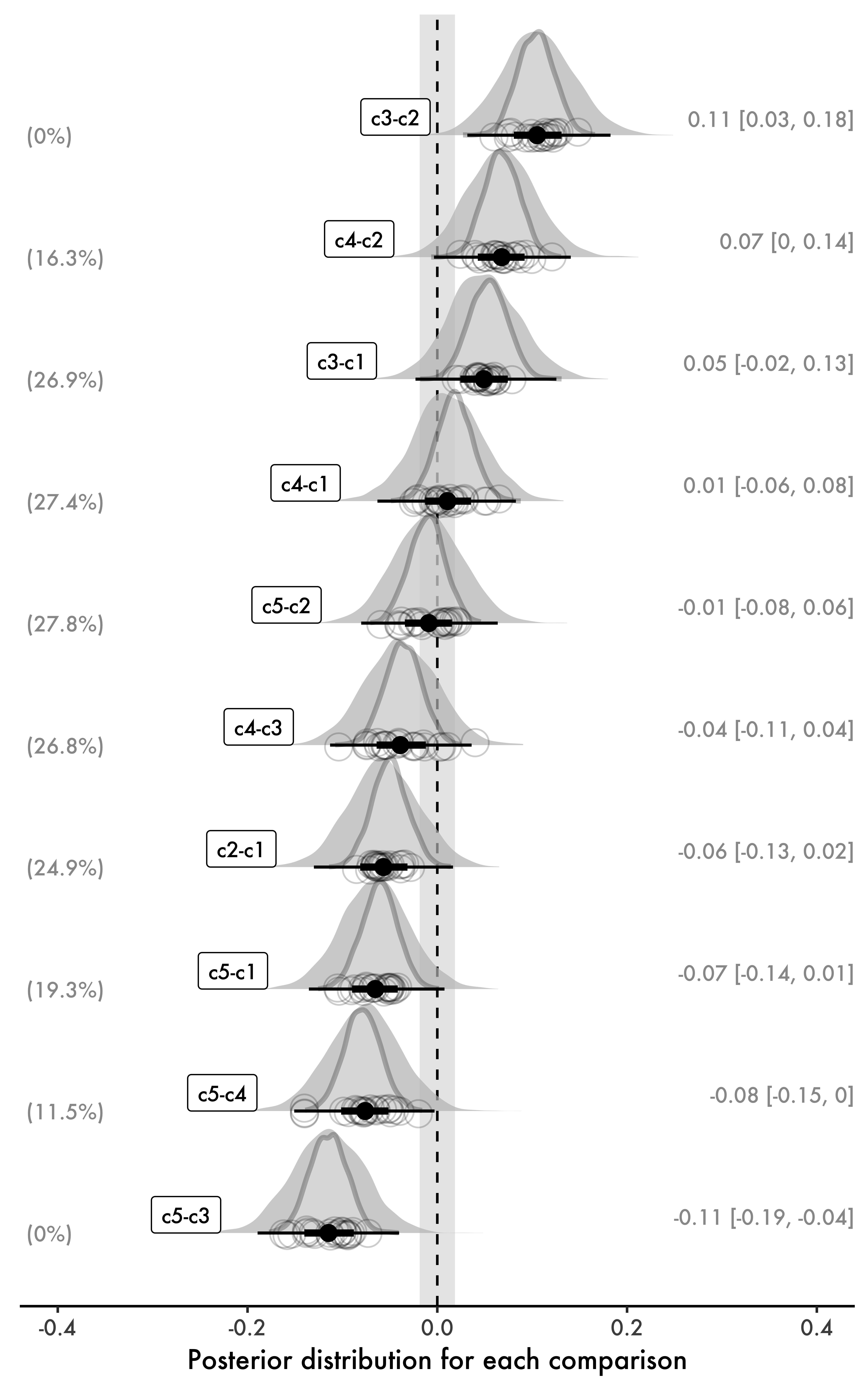
Figure 5: A complete figure containing posterior distributions of multiple comparisons using our hierarchical model. Distributions are displayed in ascending order, from lower to higher posterior means, from the bottom. Posterior distributions from a non-hierarchical model (analogous to LM in Fig. 2) are shown with dark gray borders.

At this point, the reader should immediately see the shrinkage caused by bFit1 in Fig. 5 relative to the non-hierarchical model bFit0. The priors on fixed effects used in both models are identical, which means any shrinkage due to priors can be ignored in this comparison. Thus, the only difference between the two Bayesian models is that one is hierarchical, and the other is not. Every posterior distribution involving c4, the condition with the smallest number of observations, shows considerable shrinkage: our hierarchical model is more conservative and estimates such comparisons closer to zero, which is exactly what we would expect given the shrinkage observed in the estimates of our fixed effects for c4.

By design, Fig. 5 is comprehensive in what it shows. As such, it requires multiple steps to be generated. In general, if the reader is looking for a quick method, I would recommend using the much simpler approach in Code block 9, which creates a similar result in very few steps, although that approach will be more focused on hypothesis testing. Nevertheless, as mentioned earlier, reproducing Fig. 5 can be useful to fully understand what we are doing exactly, which in turn can help us better understand the models we are using. Ultimately, it also focuses on the magnitude of effects (rather than, e.g., whether an effect is statistically different from a null model, e.g., Bayes Factors).

Below, I list the necessary steps involved in creating Fig. 5, some of which are required for both models. The reader can find a complete script to reproduce all the steps and the figure on the OSF repository mentioned at the beginning of the paper.

1. Extract draws using as_draws_df() function
2. Select and rename variables (e.g., from b_Intercept to simply c1)
3. Create comparisons
4. Long-transform the data
5. Create statistical summaries for means and HDIs using mean_hdi() function
6. Generate ROPE using rope() function
7. Extract random effects from bFit1
8. Create summary for mean (random) effects by participant
9. Generate figure

4.3 Heteroscedasticity

In our analysis above, we assume that the variance (\(\sigma^2\)), and therefore the standard deviation (\(\sigma\)), is the same across all of our conditions, i.e., they are homoscedastic. This is indeed supported by the data insofar as our conditions have very similar variances, as shown in Table 2, and therefore the variance in our residuals will be constant across all levels of cond. Sometimes, however, our conditions will not necessarily meet the assumption of equal variances. Indeed, as pointed out by Birdsong (2018, p. 1), “non-uniformity is an inherent characteristic of both early and late bilingualism”. For example, heteroscedastic data are frequently found in age effects, as older learners show higher variance than younger learners when it comes to ultimate attainment (Vanhove, 2013, p. 11).

The situation just described brings us to one additional advantage of a Bayesian approach, namely, that we can directly deal with heteroscedastic data by estimating variance itself. This provides the researcher with a higher degree of flexibility than typical Frequentist methods (e.g., robust regression models), and results in more reliable posterior distributions of effect sizes, as will be shown in below. Here, again, it is clear that more reliable posterior distributions will directly impact the reliability of multiple comparisons derived from said distributions. In this section, we will briefly see (a) how to estimate the standard deviation (\(\sigma\)) across the conditions in cond and (b) how this can affect our estimates.

The data set d_het contains a modified version of d in which the condition c4 has a considerably lower variance than all the other conditions. This can be verified in Code block 11 (cf. Table 2).

Code block 11: Modified data d_het: number of observations per condition (cond), means, variances, and standard deviations of responses (resp).

d_het |> 
  summarize(n = n(), 
            Mean = mean(resp),
            Var = var(resp),
            SD = sd(resp),
            .by = cond) |> 
  arrange(cond)
#> # A tibble: 5 × 5
#>   cond      n  Mean     Var     SD
#>   <fct> <int> <dbl>   <dbl>  <dbl>
#> 1 c1      209  6.81 0.0402  0.200 
#> 2 c2      215  6.76 0.0460  0.214 
#> 3 c3      189  6.86 0.0339  0.184 
#> 4 c4       50  6.85 0.00893 0.0945
#> 5 c5      213  6.75 0.0253  0.159

The reader can also see how the new variance of c4 affects the spread of the data, and thus the height of the box plot for c4, in Fig. 6. The figure in question can be directly compared to Fig. 1 presented at the beginning of this paper.

Figure 6: Overall patterns in the data: box plots and associated means (orange dots) and standard errors (not visible). Notice variance of c4 condition.

We will run two models. First, bFit2, which represents the same model as bFit1 run earlier. This will be a typical linear regression where we do not estimate varying standard deviations, i.e., a model that assumes homoscedasticity. We will then run bFit3, a model that estimates standard deviations (sigma) as well as the fixed and random effects estimated by bFit2. While our new model requires a new function in its specification (bf() within brm()), its interpretation is straightforward. These models will be directly comparable as they will share the same priors as well (with the exception of the prior set for sigma in bFit3). Both models, as well as the priors for bFit3, are shown in Code block 12.

Code block 12: Estimating sigma in a linear regression.

# bFit2: our "baseline" model
bFit2 = brm(resp ~ cond + (1 + cond | part) + (1 | item),
            data = d_het,
            family = gaussian(),
            cores = 4,
            prior = priors1, # same priors used for bFit1 earlier
            save_model = "bFit2.stan")

# Setting priors for bFit3:
priors2 = c(
  set_prior("normal(7, 1)", class = "Intercept"), 
  set_prior("normal(0, 1)", class = "b"),
  
  # Prior for the intercept of log(sigma)
  set_prior("normal(0, 1)", class = "Intercept", dpar = "sigma"),
  # Prior for the fixed effects of log(sigma)
  set_prior("normal(0, 1)", class = "b", dpar = "sigma"))

# bFit3: our model that also estimates sigma
bFit3 = brm(
  bf(resp ~ cond + # fixed effects
       (1 + cond | part) + (1 | item), # random effects
     sigma ~ cond), # sigma
  data = d_het,
  family = gaussian(),
  cores = 4,
  prior = priors2,
  save_model = "bFit3.stan")

The reader can see the simplified output of bFit3 in Code block 13. In addition to the estimates for cond, we also obtain estimates for \(\sigma\) for each level of cond. Recall that we assume a Gaussian distribution for the response variable. This distribution has two parameters: \(\mu\) (the mean) and \(\sigma\) (the standard deviation). In our model, the fixed effects (\(\beta\)) represent \(\mu\), while \(\sigma\) is now estimated explicitly for each level of cond. The key distinction here is that both parameters of the Gaussian distribution (\(\mu\) and \(\sigma\)) are being estimated by our model. In brms, sigma is modeled on the log scale, as reflected in Code block 13.

Code block 13: Simplified output of bFit3

summary(bFit3)$fixed |> round(2)
#>                 Estimate Est.Error l-95% CI u-95% CI Rhat Bulk_ESS Tail_ESS
#> Intercept           6.81      0.03     6.75     6.88    1  1167.26  2067.45
#> sigma_Intercept    -1.91      0.05    -2.01    -1.80    1  3147.79  2711.18
#> condc2             -0.06      0.04    -0.12     0.02    1  1856.54  2175.70
#> condc3              0.05      0.04    -0.02     0.12    1  1469.52  2120.63
#> condc4              0.04      0.04    -0.04     0.11    1  1646.49  2585.37
#> condc5             -0.07      0.03    -0.14     0.00    1  1519.37  2158.06
#> sigma_condc2        0.23      0.07     0.08     0.37    1  3564.34  3361.64
#> sigma_condc3        0.08      0.08    -0.07     0.23    1  3601.63  2917.28
#> sigma_condc4       -0.87      0.17    -1.19    -0.53    1   993.14  2073.37
#> sigma_condc5       -0.09      0.08    -0.24     0.06    1  3725.37  3145.20

To appreciate the heteroscedasticity in our data, notice how each sigma_condc... deviates from sigma_Intercept. For c1 (our intercept), the estimated log-standard deviation is \(-1.91\), which corresponds to \(\sigma_{1}=e^{-1.91} \approx 0.15\) (cf. \(0.20\) in Code block 11). For c4, the estimated log-standard deviation includes a more substantial adjustment of \(-0.87\), making \(\sigma_{4}=e^{-1.91 - 0.87} \approx 0.06\) (cf. \(0.09\) in Code block 11). We can therefore see that the estimated sigma for c4 deviates considerably from that of the intercept (c1). This reflects what we already know given Code block 11 and Fig. 6. The reader should print the outputs of both bFit2 and bFit3 to verify that the credible intervals of c4 are indeed estimated to be different in both models. Let us now examine how these differences affect our multiple comparisons. This is the goal of Fig. 7, where black point ranges represent comparisons drawn from bFit3 and orange point ranges are drawn from bFit2—mixed effects and posterior distributions are all from bFit3.

Figure 7: Multiple comparisons from a model where sigma is also estimated (black). Notice the different HDIs in comparisons involving c4 relative to a model where sigma is not estimated (orange).

In Fig. 7, we notice that comparisons involving c4 differ in their HDIs across both models. By estimating sigma, bFit3 generates narrower posteriors for c4, which the reader should verify by plotting the main effects of both models (without comparisons). This, in turn, affects the width of the posterior distributions of our comparisons in Fig. 7. For instance, in the comparison between c4 and c2, the mean effect is slightly stronger in bFit3, and its HDI now barely touches the ROPE. Another comparison worth mentioning is c4 and c5, whose HDI has clearly shifted away from the ROPE. This demonstrates how accounting for heteroscedasticity can affect both parameter estimation and hypothesis testing, emphasizing the importance of accurate variance modeling.

5 Discussion and conclusion

Let us briefly revisit the main points discussed in this tutorial. First, we reviewed why hierarchical models are often superior to non-hierarchical models. By shrinking extreme values or estimates from conditions with few observations toward the mean, hierarchical models produce more reliable and generally more conservative estimates, which in turn make derived comparisons more robust. Second, we highlighted the additional advantages of a Bayesian approach. Priors can introduce shrinkage even in non-hierarchical Bayesian models, while Bayesian flexibility allows us to estimate variance directly, addressing issues like heteroscedasticity. Finally, Bayesian models provide posterior distributions for estimates, giving us access to probability distributions of credible parameter values for multiple comparisons.

Two perspectives to data analysis were entertained in this tutorial: parameter estimation and hypothesis testing. While the former was the primary goal here, the latter is often useful and sometimes necessary, depending on our research question(s). To center our discussion on parameter estimation, we focused on credible intervals (specifically, HDIs), whose interpretation is much more intuitive than that of Frequentist confidence intervals. In the context of hypothesis testing, we considered Bayes Factors and the use of functions such as hypothesis(), as well as the use of ROPEs, which provide an additional layer of information to our figure.

Not long ago, Plonsky (2013) pointed out that research in second language acquisition relies on a narrow range of statistical methods. Fortunately, it seems that the field is slowly moving towards more comprehensive methods, such as full-fledged regression analysis with random effects (Cabrelli & Pichan, 2021; Cunnings, 2012; Garcia, 2020). Consequently, as we reduced the use of ANOVAs and post-hoc tests, multiple comparisons seem to have lost some of their popularity. In this paper, I hope to have shown how we can embrace better models and still make use of multiple comparisons when they make sense given our research questions. After all, sometimes multiple comparisons are exactly what we want in a second language study.

One key element involved in multiple comparisons when we focus on hypothesis testing is the notion of Type I error, which is based on the assumption that the null hypothesis (\(H_0\)) is true. In our scenario, under \(H_0\), the effects of our conditions would be zero (\(\beta = 0\)). While the notion of Type I error is less problematic in appropriately defined hierarchical models (e.g., Fig. 2), we should perhaps rethink the utility of the Type I error paradigm to begin with. As pointed out in Gelman et al. (2012), our starting point under this paradigm (that the effect is exactly zero) is already suboptimal: we rarely believe that an effect is exactly zero, or that there’s absolutely no differences between groups. Instead, the authors argue that the direction of an effect is a more relevant point to consider: for example, if we assume that \(\beta > 0\) but, in reality, \(\beta < 0\)—this is what Gelman & Tuerlinckx (2000) call “type S errors” (S represents the sign of an effect). In addition to type S errors, the authors propose type M errors, which pertain to the magnitude of an effect: suppose an effect is very strong but we conclude it is close to zero in an experiment. Both type S and type M errors are proposed as replacements for the Type I error paradigm, and both are, according to the proponents, “at least substantially ameliorated” in hierarchical Bayesian models (Gelman et al., 2012, p. 195).

Finally, this paper can be summarized in two recommendations for those wishing to include multiple comparisons in their analyses. First, when running regression models, we should favor hierarchical models (e.g., Barr et al., 2013) whenever appropriate given the data at hand. This decision alone already addresses several issues discussed at length in the literature of quantitative methods (Garcia, 2021; Gelman & Hill, 2006; Sonderegger, 2023; Winter, 2019), including the typical criticisms raised in the context of multiple comparisons and Type I errors (Gelman et al., 2012; Gelman & Tuerlinckx, 2000). Second, researchers should explore multiple comparisons whenever such comparisons make sense given the research question under examination. With the appropriate model, this can be accomplished without the typical corrections employed in the literature. Importantly, researchers should not fear that a Bayesian approach may be less conservative than a typical Frequentist approach: as pointed out in Gelman (2016), “[…] with normal data and a normal prior centered at 0, the Bayesian interval is always more likely to include zero, compared to the classical interval; hence we can say that Bayesian inference is more conservative, in being less likely to result in claims with confidence”.

As the models discussed in this paper become more popular in the field of second language acquisition, researchers have a lot to gain in terms of flexibility in their statistical methods—the approach presented above can be easily adapted to any Bayesian model (e.g., logistic, ordinal, and Poisson regressions). Crucially, these models provide comprehensive results that are not only more reliable, but which can also directly inform future studies through the use of priors—just as they can be informed by past research in the field.

Acknowledgments

The idea for this paper originated from a workshop I gave at the PhonLab group at Harvard during a research visit in March 2024. Thanks to Katie Franich for her comments and questions during the workshop. The visit was made possible by the Programme de mobilité professorale at Université Laval (grant number: DR140407). Thanks also to Ronaldo Lima Jr. for his comments and suggestions. Special thanks to João Veríssimo and to Rainer Düsing, whose detailed comments greatly improved this manuscript.

Copyright © 2024 Guilherme Duarte Garcia

References

Baayen, R. H. (2009). LanguageR: Data sets and functions with "analyzing linguistic data: A practical introduction to statistics". http://CRAN.R-project.org/package=languageR

Balling, L. W., & Baayen, H. R. (2008). Morphological effects in auditory word recognition: Evidence from Danish. Language and Cognitive Processes, 23(7-8), 1159–1190.

Barr, D., Levy, R., Scheepers, C., & Tily, H. (2013). Random effects structure for confirmatory hypothesis testing: Keep it maximal. Journal of Memory and Language, 68(3), 255–278.

Bates, D., & Maechler, M. (2009). lme4: Linear mixed-effects models using S4 classes. http://CRAN.R-project.org/package=lme4

Bayes, T. (1763). LII. An essay towards solving a problem in the doctrine of chances. By the late Rev. Mr. Bayes, FRS communicated by Mr. Price, in a letter to John Canton, AMFR S. Philosophical Transactions of the Royal Society of London, 53, 370–418.

Birdsong, D. (2018). Plasticity, variability and age in second language acquisition and bilingualism. Frontiers in Psychology, 9. https://doi.org/10.3389/fpsyg.2018.00081

Brand, C. O., Ounsley, J. P., Post, D. J. van der, & Morgan, T. J. H. (2019). Cumulative science via Bayesian posterior passing: An introduction. Meta-Psychology, 3.

Brooks, S., Gelman, A., Jones, G. L., & Meng, X.-L. (2011). Handbook of Markov Chain Monte Carlo. Chapman; Hall/CRC.

Bürkner, P.-C. (2016). brms: Bayesian regression models using Stan. R package version 1.5.0.

Bürkner, P.-C. (2017). brms: An R package for Bayesian multilevel models using Stan. Journal of Statistical Software, 80(1), 1–28. https://doi.org/10.18637/jss.v080.i01

Cabrelli, J., & Pichan, C. (2021). Initial phonological transfer in L3 Brazilian Portuguese and Italian. Linguistic Approaches to Bilingualism, 11(2), 131–167.

Cabrelli-Amaro, J., Flynn, S., & Rothman, J. (2012). Third language acquisition in adulthood. John Benjamins.

Carpenter, B., Gelman, A., Hoffman, M., Lee, D., Goodrich, B., Betancourt, M., Brubaker, M., Guo, J., Li, P., & Riddell, A. (2017). Stan: A probabilistic programming language. Journal of Statistical Software, Articles, 76(1), 1–32. https://doi.org/10.18637/jss.v076.i01

Cunnings, I. (2012). An overview of mixed-effects statistical models for second language researchers. Second Language Research, 28(3), 369–382. https://doi.org/10.1177/0267658312443651

Garcia, G. D. (2020). Language transfer and positional bias in English stress. Second Language Research, 36(4), 445–474. https://doi.org/10.1177/0267658319882457

Garcia, G. D. (2021). Data visualization and analysis in second language research. Routledge.

Garcia, G. D. (2023). Statistical modeling in L3/Ln acquisition. In J. Cabrelli, A. Chaouch-Orozco, J. González Alonso, S. M. Pereira Soares, E. Puig-Mayenco, & J. Rothman (Eds.), The Cambridge Handbook of Third Language Acquisition (pp. 744–770). Cambridge University Press. https://doi.org/10.1017/9781108957823.030

Gelman, A. (2008). Objections to Bayesian statistics. Bayesian Analysis, 3(3), 445–449.

Gelman, A. (2016). Bayesian inference completely solves the multiple comparisons problem. https://statmodeling.stat.columbia.edu/2016/08/22/bayesian-inference-completely-solves-the-multiple-comparisons-problem/.

Gelman, A., & Hennig, C. (2017). Beyond subjective and objective in statistics. Journal of the Royal Statistical Society Series A: Statistics in Society, 180(4), 967–1033. https://doi.org/10.1111/rssa.12276

Gelman, A., & Hill, J. (2006). Data analysis using regression and multilevel/hierarchical models. New York: Cambridge University Press.

Gelman, A., Hill, J., & Yajima, M. (2012). Why we (usually) don’t have to worry about multiple comparisons. Journal of Research on Educational Effectiveness, 5(2), 189–211.

Gelman, A., & Tuerlinckx, F. (2000). Type s error rates for classical and bayesian single and multiple comparison procedures. Computational Statistics, 15(3), 373–390.

Jaeger, T. F. (2008). Categorical data analysis: Away from ANOVAs (transformation or not) and towards logit mixed models. Journal of Memory and Language, 59(4), 434–446. https://doi.org/10.1016/j.jml.2007.11.007

Kay, M. (2020). tidybayes: Tidy data and geoms for Bayesian models. https://doi.org/10.5281/zenodo.1308151

Kruschke, J. K. (2013). Bayesian estimation supersedes the t test. Journal of Experimental Psychology: General, 142(2), 573–603.

Kruschke, J. K. (2015). Doing bayesian data analysis: A tutorial with R, JAGS, and Stan (2nd ed.). Academic Press.

Kruschke, J. K. (2021). Bayesian analysis reporting guidelines. Nature Human Behaviour, 5(10), 1282–1291.

Kruschke, J. K., & Liddell, T. M. (2018). Bayesian data analysis for newcomers. Psychonomic Bulletin & Review, 25(1), 155–177.

Luce, R. D. (1991). Response times: Their role in inferring elementary mental organization. Oxford University Press.

Makowski, D., Ben-Shachar, M. S., & Lüdecke, D. (2019). BayestestR: Describing effects and their uncertainty, existence and significance within the Bayesian framework. Journal of Open Source Software, 4(40), 1541. https://doi.org/10.21105/joss.01541

McElreath, R. (2020). Statistical rethinking: A Bayesian course with examples in R and Stan (2nd ed.). Chapman & Hall/CRC.

McGrayne, S. B. (2011). The theory that would not die: How Bayes’ rule cracked the enigma code, hunted down Russian submarines, & emerged triumphant from two centuries of controversy. Yale University Press.

Plonsky, L. (2013). Study quality in SLA: An assessment of designs, analyses, and reporting practices in quantitative L2 research. Studies in Second Language Acquisition, 35(4), 655–687.

Plonsky, L. (2014). Study quality in quantitative L2 research (1990–2010): A methodological synthesis and call for reform. The Modern Language Journal, 98(1), 450–470.

Plonsky, L., & Oswald, F. L. (2017). Multiple regression as a flexible alternative to ANOVA in L2 research. Studies in Second Language Acquisition, 39(3), 579–592. https://doi.org/10.1017/S0272263116000231

R Core Team. (2024). R: A language and environment for statistical computing. R Foundation for Statistical Computing. http://www.R-project.org/

Sonderegger, M. (2023). Regression modeling for linguistic data. MIT Press.

Vanhove, J. (2013). The critical period hypothesis in second language acquisition: A statistical critique and a reanalysis. PloS One, 8(7), e69172.

Veríssimo, J. (2024). A gentle introduction to Bayesian statistics, with applications to bilingualism research. PsyArXiv. https://doi.org/10.31234/osf.io/7wfus

Whelan, R. (2008). Effective analysis of reaction time data. The Psychological Record, 58, 475–482.

Wickham, H., Averick, M., Bryan, J., Chang, W., McGowan, L. D., François, R., Grolemund, G., Hayes, A., Henry, L., Hester, J., Kuhn, M., Pedersen, T. L., Miller, E., Bache, S. M., Müller, K., Ooms, J., Robinson, D., Seidel, D. P., Spinu, V., … Yutani, H. (2019). Welcome to the tidyverse. Journal of Open Source Software, 4(43), 1686. https://doi.org/10.21105/joss.01686

Winter, B. (2019). Statistics for linguists: An introduction using R. Routledge.

Footnotes

1. This is not a strict rule, as confidence intervals in hierarchical models may also be narrower than those in non-hierarchical models, depending on the structure of the data. Similarly, while the standard errors in our hierarchical model are greater than those in the two non-hierarchical models—a common characteristic of hierarchical models—this is not universally the case.

2. The set of possible values for a given variable, e.g., a coefficient in a regression model.

3. Recall that resp has been log-transformed, as is typical for reaction time data.

4. While this is good news given the notion of homoscedasticity, Bayesian models make it much easier for us to assume difference variances across groups. This is not discussed here but is yet another advantage of Bayesian data analysis.

5. Unlike in Frequentist statistics, in a Bayesian posterior distribution, the standard error is equivalent to the standard deviation.

6. Also known as the Gelman-Rubin convergence diagnostic; see Brooks et al. (2011).

7. This is indeed what is done for our null model bFitNull in Code block 5 above, since ESS values are too low with the default number of iterations.

8. Not to be confused with the Frequentist \(\alpha\) level, which represents the long-run probability of making a Type I error, a meaning that is tied to the concept of repeated sampling.

9. By default, the function uses 90% credible intervals for one-sided and 95% credible intervals for two-sided hypotheses—note that these are not highest density intervals. The reader should consult the documentation for the hypothesis() function to read more about its assumptions and its output.

10. This, of course, depends on the contrasts used in the model, which can be changed.

11. Just like in any interval, 95% is an arbitrary threshold.

12. We will see more effects if we consider all possible comparisons, as shown in Fig. 5.

13. Notice that you can easily plot the comparisons using |> plot(), commented out in the code. This will generate a standard ggplot2 figure.