pak::pak("guilhermegarcia/Fonology")Phonology from text
the Fonology package for R
Fonology
corpus
maxent
SSHRC
CRSH
TipThe role of lexical and post-lexical statistics in second language acquisition
How can we map phonological patterns in a language using written data?
We see text everywhere, so it’s reasonable to assume that gathering data has never been easier. The problem is the well-known mismatch between letters (graphemes) and sounds (phonemes): we cannot fully understand phonological systems by simply examining how letters are distributed in a given corpus. Thus, to map phonological patterns, we first need to convert graphemes into phonemes.
This series is dedicated to a SSHRC-funded project (grant no. 141280) examining how lexical statistics can be explored to generate a baseline for comparison with experimental data. Part of this project involves the development of grapheme-phoneme conversion tools — it is very difficult to examine phonological patterns in written data without access to phonetic transcription. The Fonology package is directly connected to this project, covering Portuguese, French, Italian, and Spanish. English (demoed below) was added to the list of supported languages in 2026.
Fonology for R
Fonology is a package I’ve been working on since 2023, when it supported only Portuguese. In a nutshell, it allows you to extract phonological variables from written data. The package now supports English (as of 2026), French, Italian, Portuguese and Spanish, with different levels of grapheme-phoneme conversion accuracy.1 The demo below is based on a seminar I gave at Universidad de Granada in April 2026 as part of the Erasmus+ program (partnership between Université Laval and Universidad Granada). The goal here is simple: take written data, extract phonological variables, run a MaxEnt model to learn weights. This illustrates how Fonology can be used to a) transcribe text in multiple languages, b) extract a wide range of variables, and c) run probabilistic grammars. You can access the package here, where you can learn about all the available functions. The short demo below is only a subset of what the package can do, but it’s probably the quickest way to understand why the package exists.
Demo
Let’s go over a sequence of steps that demonstrate how Fonology can be used with two texts, one in English (Moby Dick) and one in Portuguese (Memórias Póstumas de Brás Cubas). To illustrate different functions in the package, we will follow these steps:
- Phonemically transcribe both texts
- Extract syllable shapes
- Run a MaxEnt grammar for both languages (Goldwater and Johnson 2003; Hayes and Wilson 2008)
- Plot constraint weights by language
Step 0: Install packages
We’ll be using tidyverse, gutenbergr, tidytext and Fonology below. Make sure you have all these packages installed. To install Fonology, you can use pak (but you’ll have to install pak first).
Once you have all the packages in question, you’ll be ready to move on to step 1 below.
Step 1: Load texts
You can use gutenbergr to download both novels from the Gutenberg project. This step also saves both texts into a single RData file.
library(gutenbergr)
library(Fonology)
library(tidyverse)
library(tidytext)

# Download Moby Dick
1gutenberg_metadata |>
  filter(author == "Melville, Herman") |>
  select(gutenberg_id, title) |>
  print(n = 20)

2moby_raw <- gutenberg_download(2701) |> select(text)

# Download Brás Cubas
gutenberg_metadata |>
  filter(author == "Machado de Assis") |>
  select(gutenberg_id, title) |>
  print(n = 20)

braz_raw <- gutenberg_download(54829) |> select(text)

3save(moby_raw, braz_raw, file = "texts.RData")- 1
- This allows us to print some books (and their IDs) by Melville to make sure the target text exists
- 2
- We can then download Moby Dick by using its ID number
- 3
-
Finally, we save everything into an
RDatafile
Step 2: Tokenize & code
Now that we’ve saved our texts, we won’t need to redownload the data next time. The code below assumes a different session to demonstrate how to load the RData file in question. To demonstrate how syllabic constituents can be extracted, the code below also takes the onset of the final syllable.
load("texts.RData")
md <- moby_raw |>
  unnest_tokens(word, text) |>
  filter(
1    !word %in% stopwords_en
  ) |>
2  mutate(
    ipa = ipa(word, lg = "en"),
    cv = cv(ipa),
    weight = getWeight(ipa, lg = "en"),
    stress = getStress(ipa),
    finSyl = getSyl(ipa, 1),
    onsetFin = syllable(finSyl, const = "onset", glides_as_onsets = TRUE)
  )

bc <- braz_raw |>
  unnest_tokens(word, text) |>
  filter(
    !word %in% stopwords_pt
  ) |>
  mutate(
    ipa = ipa(word, lg = "pt"),
    cv = cv(ipa),
    weight = getWeight(ipa, lg = "pt"),
    stress = getStress(ipa),
    finSyl = getSyl(ipa, 1),
    onsetFin = syllable(finSyl, const = "onset", glides_as_onsets = TRUE)
)- 1
-
Remove stopwords from text (the same is used for the Portuguese text). This is a list of words included in
Fonologyfor all supported languages; the lists come from thestopwordspackage - 2
-
This is where most of the work takes place. We’re adding several columns that code for different phonological variables: transcription, CV shape, weight, stress, the final syllable, and the onset of that syllable. These are all functions in
Fonology
Below, you can see the resulting tibbles. For English, the function ipa() first uses the CMU Dictionary as a lookup. Next, it checks a second database for specific words (a custom lexicon). Finally, words that don’t exist in either database are transcribed using a series of rules. Because grapheme-phoneme conversion in English is not very reliable, all words whose IPA transcription is derived by rules end with an asterisk, so you can easily check or remove them if you want to. For Moby Dick, only 2% of tokens fall into that category. For the other languages supported in Fonology, transcription is rule-based. Lines containing only numbers are coded as NA (e.g., chapter numbers).
md # Moby Dick# A tibble: 81,958 × 7
word ipa cv weight stress finSyl onsetFin
<chr> <chr> <chr> <chr> <chr> <chr> <chr>
1 moby ˈmoʊ.bi CVV.CV HL penult bi b
2 dick ˈdɪk CVC H final dɪk d
3 whale ˈweɪl GVVC H final weɪl w
4 herman ˈhɝ.mən CV.CVC LH penult mən m
5 melville ˈmɛl.vɪl CVC.CVC HH penult vɪl v
6 contents ˈkɑn.tɛnts CVC.CVCCC HH penult tɛnts t
7 etymology ɛ.tə.ˈmɑ.lə.dʒi V.CV.CV.CV.CCV LLL antepenult dʒi dʒ
8 extracts ˈɛks.tɹækts VCC.CCVCCC HH penult tɹækts tɹ
9 supplied sə.ˈplaɪd CV.CCVVC LH final plaɪd pl
10 librarian laɪ.ˈbɹɛ.ɹi.ən CVV.CCV.CV.VC LLH antepenult ən <NA>
# ℹ 81,948 more rowsbc # Brás Cubas# A tibble: 29,239 × 7
word ipa cv weight stress finSyl onsetFin
<chr> <chr> <chr> <chr> <chr> <chr> <chr>
1 memórias me.ˈmɔ.ri.as CV.CV.CV.VC LLH antepenult as <NA>
2 pósthumas ˈpɔs.tu.mas CVC.CV.CVC HLH antepenult mas m
3 braz ˈbras CCVC H final bras br
4 cubas ˈku.bas CV.CVC LH penult bas b
5 machado ma.ˈʃa.do CV.CV.CV LLL penult do d
6 assis a.ˈsis V.CVC LH final sis s
7 rio ˈxi.o CV.V LL penult o <NA>
8 janeiro ʒa.ˈnej.ro CV.CVG.CV LHL penult ro r
9 typographia ti.po.gra.ˈpi.a CV.CV.CCV.CV.V LLL penult a <NA>
10 nacional na.si.o.ˈnal CV.CV.V.CVC LLH final nal n
# ℹ 29,229 more rowsStep 3: Phonotactics
Next, we split words into syllables because we don’t care about the position of each CV shape for this demo. This results in a modified cv column where each row contains only one syllable. Consequently, our tibbles will be longer now — see outputs below. We will now be able to calculate which syllable shapes are the most common across both languages using these texts as references.
md_phon <- md |>
  separate_rows(cv, sep = "\\.")
# # A tibble: 151,453 × 7
#    word     ipa        cv    weight stress finSyl onsetFin
#    <chr>    <chr>      <chr> <chr>  <chr>  <chr>  <chr>
#  1 moby     ˈmoʊ.bi    CVV   HL     penult bi     b
#  2 moby     ˈmoʊ.bi    CV    HL     penult bi     b
#  3 dick     ˈdɪk       CVC   H      final  dɪk    d
#  4 whale    ˈweɪl      GVVC  H      final  weɪl   w
#  5 herman   ˈhɝ.mən    CV    LH     penult mən    m
#  6 herman   ˈhɝ.mən    CVC   LH     penult mən    m

bc_phon <- bc |>
  separate_rows(cv, sep = "\\.")
# # A tibble: 80,910 × 7
#    word      ipa          cv    weight stress     finSyl onsetFin
#    <chr>     <chr>        <chr> <chr>  <chr>      <chr>  <chr>
#  1 memórias  me.ˈmɔ.ri.as CV    LLH    antepenult as     <NA>
#  2 memórias  me.ˈmɔ.ri.as CV    LLH    antepenult as     <NA>
#  3 memórias  me.ˈmɔ.ri.as CV    LLH    antepenult as     <NA>
#  4 memórias  me.ˈmɔ.ri.as VC    LLH    antepenult as     <NA>
#  5 pósthumas ˈpɔs.tu.mas  CVC   HLH    antepenult mas    m
#  6 pósthumas ˈpɔs.tu.mas  CV    HLH    antepenult mas    m
To simplify the comparison between English and Portuguese, let’s focus on the most representative syllable shapes. The code below filters the data and calculates the proportions we will need for our MaxEnt analysis later.
# MOBY DICK:
md_phon |>
  distinct() |>
  filter(cv %in% c("CCV", "CV", "V", "VC", "CVC", "VCC", "CVCC", "CCVCC")) |>
  summarize(
    obs = n(), .by = cv
  ) |>
  mutate(
    prop = obs / sum(obs)
  )
# # A tibble: 8 × 3
#   cv      obs   prop
#   <chr> <int>  <dbl>
# 1 CV     7345 0.301
# 2 CVC    7738 0.317
# 3 V      1633 0.0670
# 4 CCV    1843 0.0756
# 5 VCC     460 0.0189
# 6 VC     2217 0.0910
# 7 CVCC   2556 0.105
# 8 CCVCC   580 0.0238

# BRÁS CUBAS:
bc_phon |>
  distinct() |>
  filter(cv %in% c("CCV", "CV", "V", "VC", "CVC", "VCC", "CVCC", "CCVCC")) |>
  summarize(
    obs = n(), .by = cv
  ) |>
  mutate(
    prop = obs / sum(obs)
  )
# # A tibble: 8 × 3
#   cv      obs    prop
#   <chr> <int>   <dbl>
# 1 CV     8285 0.444
# 2 VC     1639 0.0878
# 3 CVC    5073 0.272
# 4 V      2142 0.115
# 5 CCV    1382 0.0740
# 6 CVCC     89 0.00477
# 7 VCC      28 0.00150
# 8 CCVCC    37 0.00198
Step 4: MaxEnt
Finally, using the summaries created above, we can now generate our tableaux using the tribble() function. We need columns for input, output, the constraints, and the number of observed outputs. To keep the illustration simple, let’s assume the following constraints: onset, no_coda, no_complex_onset.
tableau_md <- tribble(
  ~input, ~output, ~onset, ~no_coda, ~no_complex_onset, ~obs,
  "input", "CV", 0, 0, 0, 7345,
  "input", "CVC", 0, 1, 0, 7738,
  "input", "V", 1, 0, 0, 1633,
  "input", "CCV", 0, 0, 1, 1843,
  "input", "VCC", 1, 2, 0, 460,
  "input", "VC", 1, 1, 0, 2217,
  "input", "CVCC", 0, 2, 0, 2556,
  "input", "CCVCC", 0, 2, 1, 580,
)

tableau_bc <- tribble(
  ~input, ~output, ~onset, ~no_coda, ~no_complex_onset, ~obs,
  "input", "CV", 0, 0, 0, 8285,
  "input", "VC", 1, 1, 0, 1639,
  "input", "CVC", 0, 1, 0, 5073,
  "input", "V", 1, 0, 0, 2142,
  "input", "CCV", 0, 0, 1, 1382,
  "input", "CVCC", 0, 2, 0, 89,
  "input", "VCC", 1, 2, 0, 28,
  "input", "CCVCC", 0, 2, 1, 37,
)
Once we copy the number of observations from the summaries above, we’re ready to use the maxent() function. By default, the function returns multiple elements, but the two most important ones are predictions and weights. Because the output is a list, you can access these elements using $.
maxent(tableau_md)$predictions
# A tibble: 8 × 13
input output onset no_coda no_complex_onset obs harmony max_h exp_h Z
<chr> <chr> <dbl> <dbl> <dbl> <dbl> <dbl> <dbl> <dbl> <dbl>
1 input CV 0 0 0 7345 0 2.49 12.0 34.3
2 input CVC 0 1 0 7738 0.439 2.49 7.76 34.3
3 input V 1 0 0 1633 1.41 2.49 2.94 34.3
4 input CCV 0 0 1 1843 1.61 2.49 2.41 34.3
5 input VCC 1 2 0 460 2.29 2.49 1.22 34.3
6 input VC 1 1 0 2217 1.85 2.49 1.90 34.3
7 input CVCC 0 2 0 2556 0.878 2.49 5.00 34.3
8 input CCVCC 0 2 1 580 2.49 2.49 1 34.3
# ℹ 3 more variables: obs_prob <dbl>, pred_prob <dbl>, error <dbl>
$weights
onset no_coda no_complex_onset
1.4090772 0.4389564 1.6100479
$log_likelihood
[1] -42998.96
$log_likelihood_norm
[1] -5374.87
$bic
[1] -85991.67maxent(tableau_bc)$predictions
# A tibble: 8 × 13
input output onset no_coda no_complex_onset obs harmony max_h exp_h Z
<chr> <chr> <dbl> <dbl> <dbl> <dbl> <dbl> <dbl> <dbl> <dbl>
1 input CV 0 0 0 8285 0 4.15 63.7 128.
2 input VC 1 1 0 1639 2.35 4.15 6.10 128.
3 input CVC 0 1 0 5073 1.09 4.15 21.5 128.
4 input V 1 0 0 2142 1.26 4.15 18.0 128.
5 input CCV 0 0 1 1382 1.98 4.15 8.76 128.
6 input CVCC 0 2 0 89 2.17 4.15 7.27 128.
7 input VCC 1 2 0 28 3.43 4.15 2.06 128.
8 input CCVCC 0 2 1 37 4.15 4.15 1 128.
# ℹ 3 more variables: obs_prob <dbl>, pred_prob <dbl>, error <dbl>
$weights
onset no_coda no_complex_onset
1.261392 1.085006 1.983917
$log_likelihood
[1] -28335.66
$log_likelihood_norm
[1] -3541.957
$bic
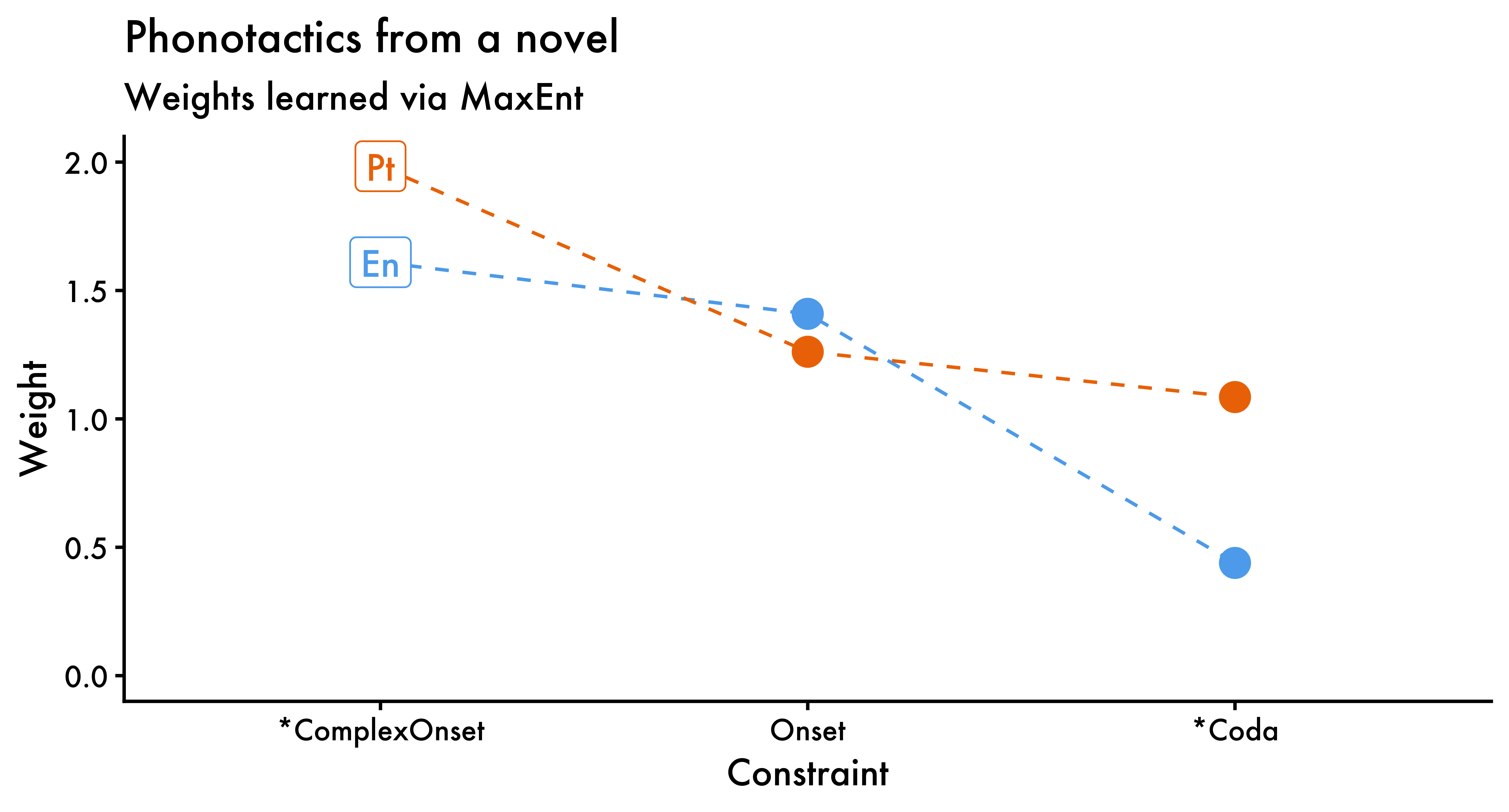
[1] -56665.07Unsurprisingly, both no_coda and no_complex_onset have higher weights in Portuguese than in English. Finally, while it’s not very common to visualize MaxEnt weights, we can easily do that to better appreciate how both languages differ vis-à-vis their phonotactics (at least given the data analyzed here).
1weights_en <- tableau_md |>
  maxent() |>
  _$weights

weights_pt <- tableau_bc |>
  maxent() |>
  _$weights

2weights <- tibble(
  lang = rep(c("En", "Pt"), each = length(weights_pt)),
  constraint = rep(names(weights_pt), times = 2),
  weight = c(weights_en, weights_pt)
)

ggplot(data = weights,
  aes(x = reorder(constraint, -weight),
    y = weight,
    color = lang)) +
  geom_line(aes(group = lang, color = lang), linetype = "dashed") +
  geom_point(size = 4) +
3  geom_label(data = weights |>
    filter(constraint == "no_complex_onset"),
    aes(label = lang)) +
  theme_classic(base_family = "Futura") +
  theme(legend.position = "none") +
  labs(
    x = "Constraint", y = "Weight", color = "Language:",
    title = "Phonotactics from a novel",
    subtitle = "Weights learned via MaxEnt"
  ) +
  scale_colour_manual(
    values = c("steelblue2", "darkorange2")
  ) +
  scale_x_discrete(
    labels = c(
      no_coda = "*Coda",
      onset = "Onset",
      no_complex_onset = "*ComplexOnset"
    )
  ) +
coord_cartesian(ylim = c(0, 2))- 1
- Extract weights from tableaux
- 2
- Create tibble with data to be plotted2
- 3
- Identify language with labels
Copyright © Guilherme Duarte Garcia
References
Goldwater, Sharon, and Mark Johnson. 2003. “Learning OT Constraint Rankings Using a Maximum Entropy Model.” Proceedings of the Stockholm Workshop on Variation Within Optimality Theory, 111–20.
Hayes, Bruce, and Colin Wilson. 2008. “A Maximum Entropy Model of Phonotactics and Phonotactic Learning.” Linguistic Inquiry 39 (3): 379–440. https://doi.org/10.1162/ling.2008.39.3.379.
Footnotes
You will notice mismatches at times, especially if you’re transcribing older texts, which tend to be based on older orthographic patterns. You can see an example below: typographia in Portuguese, which is now written as tipografia. This is all to say that accuracy will not be 100%, but it will be above 80-85% based on samples I’ve tested in the recent past. For English, accuracy will be much higher, as it uses lookups (certainly above 90%).↩︎
While it’s typically not recommended to connect categories across the x-axis with lines, a dashed line here makes the figure easier to read.↩︎