pak::pak("guilhermegarcia/fonology")
# Alternatively:
remotes::install_github("guilhermegarcia/fonology")Fonology package
Phonological Analysis in R
 The
The Fonology package (Garcia, 2026) provides different functions that are relevant to phonology research and/or teaching. If you have any suggestions or feedback, please visit the GitHub page of the project. There you will find a discussions page for general questions. Please, feel free to open an issue to help improve the package. To install the package, use one of the commands below.
![]()
![]()


TipVersion 1.2.0 is here
All five languages now use lexical lookup before falling back to regular-expression rules: new Wiktionary-derived lexicons were added for Italian (~82K words) and Spanish (~130K words), joining the existing English (CMU), French (Lexique 4), and Portuguese (PSL) lookups. Words not found in a lexicon are transcribed by rules and marked with a final *, and the rule-based fallbacks were substantially improved for all languages (see the accuracy table below). User-defined entries from add_lex_pt() and friends take priority over everything else.
ImportantShiny App now available: text2ipa
If you’re not familiar with R, try out the new app text2ipa here. It allows you to phonemically transcribe text and generate tables with phonological variables for all five languages supported in Fonology.
How to install
Main functions and data
ipa()phonemically transcribes words (real or not) in English, French, Italian, Portuguese and SpanishgetFeat()andgetPhon()to work with distinctive featuressyllable()extracts syllabic constituentsmaxent()builds a MaxEnt Grammar (see alsonhg())sonDisp()calculates the sonority dispersion of a given demisyllable or the average dispersion for a set of words—see alsomeanSonDisp()for the average dispersion of a given wordplotSon()plots the sonority profile of a given wordbiGram_pt()calculates bigram probabilities for a given wordwug_pt()generates hypothetical words in PortugueseplotVowels()generates vowel trapezoidsipa2tipa()translates IPA sequences intotipasequences (also seeipa2typst())monthsAge()andmeanAge()add_lex_pt()and its siblings (_en,_fr,_it,_sp) let you add your own entries to the lexicons used byipa(); see alsoremove_lex_pt()(and siblings) andexport_lex()pslcontains the Portuguese Stress Lexiconpt_lexcontains a simplified version ofpslen_lex,fr_lex,it_lex, andsp_lexcontain the lookup lexicons used byipa(): CMU-derived for English, Lexique 4-derived for French, and Wiktionary-derived (via Wiktextract/kaikki.org) for Italian and Spanishstopwords_pt,stopwords_en,stopwords_fr,stopwords_it, andstopwords_spcontain stopwords in Portuguese, English, French, Italian and Spanish
IPA transcription
The function ipa() takes a word (or a vector with multiple words, real or not) in its orthographic form and returns its phonemic (i.e., broad) transcription, including syllabification and stress. Five languages are currently supported: English, French, Italian, Portuguese, and Spanish. All five languages use lexical lookup first: words found in the language’s lexicon get their dictionary transcription, and only out-of-vocabulary words (nonce words, rare forms, names) are transcribed by regular-expression rules. Rule-derived transcriptions are marked with a final *—helper functions ignore this marker, so it’s safe to pipe starred forms into the rest of the package. Narrow transcription is available for Portuguese (based on Brazilian Portuguese), which includes secondary stress—this can be generated by adding narrow = T to the function. Run ipa_pt_test(), ipa_en_test(), ipa_fr_test(), ipa_it_test(), and ipa_sp_test() for sample words. By default, ipa() assumes that lg = "Portuguese" (or lg = "pt") and narrow = F.
library(Fonology)
ipa("comfortably", lg = "en")
#> [1] "ˈkʌm.fɚ.tə.bli"
ipa("atlético")
#> [1] "a.ˈtlɛ.ti.ko"
ipa("antidepressivo", narrow = T)
#> [1] "ˌãn.t͡ʃi.ˌde.pɾe.ˈsi.vʊ"
ipa("nuevos", lg = "sp")
#> [1] "ˈnwe.bos"
ipa("informatique", lg = "fr")
#> [1] "ɛ̃.fɔʁ.ma.tik"
ipa("stazione", lg = "it")
#> [1] "stat.ˈtsjo.ne"
ipa("blimpo")           # nonce word: rule-based fallback, marked with *
#> [1] "ˈblim.po*"
How much can you trust each path? Lookup transcriptions are dictionary-grade by construction. The rule-based fallbacks are benchmarked against 4,000 held-out words from each language’s lexicon (exact match, including stress and syllabification); token coverage is measured on running-text samples. Note the two-way trade-off: languages with shallow orthographies (Spanish, Portuguese) barely need their lexicons, while English relies almost entirely on lookup.
| Language | Lookup source | Entries | Token coverage | Fallback (exact) | Overall |
|---|---|---|---|---|---|
| English | CMU Pronouncing Dictionary | ~133K | ~99.9% | 27% | ~99.9% |
| French | Lexique 4 | ~171K | ~99% | 71% | ~99% |
| Spanish | Wiktionary (kaikki.org) | ~130K | ~83% | 95% | ~98% |
| Italian | Wiktionary (kaikki.org) | ~82K | ~92% | 70% | ~97% |
| Portuguese | Portuguese Stress Lexicon | ~129K | ~25% | 95% | ~94% |
| Spanish coverage measured on a classical text; modern text runs higher. The PSL contains non-verbs only, so Portuguese function words and verbs are served by the (near-dictionary-accurate) fallback. | |||||
Customizing transcriptions
If a transcription comes out wrong—or a loanword resists the rules—you can add your own entries, which take priority over both the lexicon and the fallback. Entries persist in your local installation across sessions.
# Portuguese, Spanish, Italian: diacritized forms fix stress/vowel quality
add_lex_it("chièdere")            # è marks stress + open-mid vowel
# Or store an exact IPA transcription for any language:
add_lex_pt("shampoo", ipa = "ʃam.ˈpu")
add_lex_en("naive", ipa = "na.ˈiv")
ipa("shampoo")                    # returns ʃam.ˈpu verbatim
export_lex("pt", "my_ipa.tsv", ipa = TRUE)  # share your IPA entries
WarningA note on reproducibility
Entries added with add_lex_*() are stored on your machine (under tools::R_user_dir()), not in your script. For any analysis you intend to share or publish, declare your entries at the top of the script—calls are idempotent, so re-running is safe—or ship them with export_lex(). And if a common word is mistranscribed, please open an issue instead: the fix then benefits everyone.
Helper functions
If you plan to tokenize texts and create a table with individual columns for stress and syllables, you can use some simple additional helper functions. For example, getWeight() will take a syllabified word and return its weight profile (e.g., getWeight("kon.to") will return HL). The function getStress() will return the stress position of a given word (up to preantepenultimate stress)—the word must already be stressed, but the symbol used can be specified in the function (argument stress). The function can instead extract the stressed syllable with the argument syl = TRUE. Finally, countSyl() will return the number of syllables in a given string, and getSyl() will extract a particular syllable from a string. For example, getSyl(word = "kom-pu-ta-doɾ", pos = 3, syl = "-") will take the antepenultimate syllable of the string in question (you can set the direction of the parsing with the argument dir). The default symbol for syllabification is the period.
Here’s a simple example of how you could tokenize a text and create a table with coded variables using the functions discussed thus far (and without using packages such as tm or tidytext)—note also the function cleanText().
library(tidyverse)
text = "Por exemplo, em quase todas as variedades do português..."

d = tibble(word = text |>
             cleanText())

d = d |>
  mutate(IPA = ipa(word),
         stress = getStress(IPA),
         weight = getWeight(IPA),
         syl3 = getSyl(IPA, 3),
         syl2 = getSyl(IPA, 2),
         syl1 = getSyl(IPA, 1),
         syl_st = getStress(IPA, syl = TRUE)) |> # get stressed syllable
filter(!word %in% stopwords_pt) # remove stopwords| word | IPA | stress | weight | syl3 | syl2 | syl1 | syl_st |
|---|---|---|---|---|---|---|---|
| quase | ˈkwa.ze* | penult | LL | NA | kwa | ze | kwa |
| variedades | va.ri.e.ˈda.des* | penult | LLH | e | da | des | da |
| português | por.tu.ˈges | final | HLH | por | tu | ges | ges |
We often need to extract onsets, nuclei, codas and rhymes from syllables. That’s what syllable() does: given a syllable (phonemically transcribed), the function returns a constituent of interest. Let’s add columns to d where we extract all constituents of the final syllable (syl1 column).
d = d |>
  select(-c(syl3, syl2, stress)) |>
  mutate(on1 = syllable(syl = syl1, const = "onset"),
         nu1 = syllable(syl = syl1, const = "nucleus"),
         co1 = syllable(syl = syl1, const = "coda"),
rh1 = syllable(syl = syl1, const = "rhyme"))| word | IPA | weight | syl1 | syl_st | on1 | nu1 | co1 | rh1 |
|---|---|---|---|---|---|---|---|---|
| quase | ˈkwa.ze* | LL | ze | kwa | z | e | NA | e |
| variedades | va.ri.e.ˈda.des* | LLH | des | da | d | e | s | es |
| português | por.tu.ˈges | HLH | ges | ges | g | e | s | es |
It’s important to decide whether we want to count glides as part of onsets or codas, or whether we want them to be included in nuclei only. By default, syllable() assumes that all glides are nuclear. You can change that by setting glides_as_onsets = T and glides_as_codas = T (both are set to F by default).
TipDo you have tons of data?
If you have a considerably large number of words to analyze with functions such as ipa() or syllable(), it’s much faster to first run the functions on types and then extend the variables created to all tokens (say, by using right_join() from dplyr).
IPA transcription of lemmas
You can easily combine Fonology with other packages that have tagging capabilities. In the example below, we import a short excerpt of Os Lusíadas, tag it using udpipe (Wijffels, 2023), and transcribe only the nouns in the data.
library(udpipe)
udpipe_model_file = "portuguese-gsd-ud-2.5-191206.udpipe"

if (!file.exists(udpipe_model_file)) {
  # Download the model once, then reuse the local file on future renders.
  udpipe_download_model(language = "portuguese-gsd")
}

udmodel_pt = udpipe_load_model(file = udpipe_model_file)

txt_pt = read_lines("data_files/lus.txt") |>
  str_to_lower()

set.seed(1)
annotation_pt = udpipe_annotate(udmodel_pt, txt_pt) |>
  as_tibble() |>
  select(sentence, token, lemma, upos)

lusiadas = annotation_pt |>
  select(lemma, upos) |>
  filter(upos == "NOUN",
         !is.na(lemma)) |>
  mutate(ipa = ipa(lemma),
         stress = getStress(ipa)) |>
  select(-upos) |>
ungroup()| lemma | ipa | stress |
|---|---|---|
| arma | ˈar.ma | penult |
| barão | ba.ˈrãw̃ | final |
| praia | ˈpra.ja | penult |
| mar | ˈmar* | final |
| taprobana | ta.pro.ˈba.na* | penult |
Probabilistic grammars
The function maxent() estimates weights in a Maximum Entropy Grammar (Goldwater & Johnson, 2003; Hayes & Wilson, 2008; Wilson, 2006) given a tableau object containing inputs, outputs, constraints, violations and observations (see documentation). The function returns a list with different objects, including learned weights, BIC value and predicted probabilities for each output. If the reader wishes to pursue a comprehensive MaxEnt analysis, I strongly recommend the maxent.ot package, which is dedicated exclusively to MaxEnt grammars (Mayer et al., 2024). Here’s an example of maxent() in action.
maxent_data <- tibble::tibble(
  input = rep(c("pad", "tab", "bid", "dog", "pok"), each = 2),
  output = c("pad", "pat", "tab", "tap", "bid", "bit", "dog", "dok", "pog", "pok"),
  ident_vce = c(0, 1, 0, 1, 0, 1, 0, 1, 1, 0),
  no_vce_final = c(1, 0, 1, 0, 1, 0, 1, 0, 1, 0),
  obs = c(5, 15, 10, 20, 12, 18, 12, 17, 4, 8)
)
maxent(tableau = maxent_data)
#> $predictions
#> # A tibble: 10 × 12
#>    input output ident_vce no_vce_final   obs harmony max_h exp_h     Z obs_prob
#>    <chr> <chr>      <dbl>        <dbl> <dbl>   <dbl> <dbl> <dbl> <dbl>    <dbl>
#>  1 pad   pad            0            1     5  0.639  0.639  1     2.79    0.25
#>  2 pad   pat            1            0    15  0.0541 0.639  1.79  2.79    0.75
#>  3 tab   tab            0            1    10  0.639  0.639  1     2.79    0.333
#>  4 tab   tap            1            0    20  0.0541 0.639  1.79  2.79    0.667
#>  5 bid   bid            0            1    12  0.639  0.639  1     2.79    0.4
#>  6 bid   bit            1            0    18  0.0541 0.639  1.79  2.79    0.6
#>  7 dog   dog            0            1    12  0.639  0.639  1     2.79    0.414
#>  8 dog   dok            1            0    17  0.0541 0.639  1.79  2.79    0.586
#>  9 pok   pog            1            1     4  0.693  0.693  1     3.00    0.333
#> 10 pok   pok            0            0     8  0      0.693  2.00  3.00    0.667
#> # ℹ 2 more variables: pred_prob <dbl>, error <dbl>
#>
#> $weights
#>    ident_vce no_vce_final
#>   0.05410682   0.63904035
#>
#> $log_likelihood
#> [1] -78.72152
#>
#> $log_likelihood_norm
#> [1] -7.872152
#>
#> $bic
#> [1] -152.8379
Finally, a couple of functions are dedicated to Noisy Harmonic Grammars. These are pedagogical tools that can be used to demonstrate how probabilities are generated given constraint weights and violation profiles for different candidates. The function nhg() takes a tableau object and returns predicted probabilities given n simulations. The user can also set the standard deviation for the noise used. The function plotNhg() can be helpful to visualize how different standard deviations affect probabilities over candidates after 100 simulations.
Distinctive features
The function getFeat() requires a set of phonemes ph and a language lg. It outputs the minimal matrix of distinctive features for ph given the phonemic inventory of lg. Five languages are supported: English, French, Italian, Portuguese, and Spanish. You can also use a custom phonemic inventory. See examples below.
The function getPhon() requires a feature matrix ft (a simple vector in R) and a language lg. It outputs the set of phonemes represented by ft given the phonemic inventory of lg. The languages supported are the same as those supported by getFeat(), and you can again provide your own phonemic inventory.
library(Fonology)

getFeat(ph = c("i", "u"), lg = "English")
#> [1] "+hi"    "+tense"
getFeat(ph = c("i", "u"), lg = "French")
#> [1] "Not a natural class in this language."
getFeat(ph = c("i", "y", "u"), lg = "French")
#> [1] "+syl" "+hi"
getFeat(ph = c("p", "b"), lg = "Portuguese")
#> [1] "-son"  "-cont" "+lab"
getFeat(ph = c("k", "g"), lg = "Italian")
#> [1] "+cons" "+back"library(Fonology)
getPhon(ft = c("+syl", "+hi"), lg = "French")
#> [1] "u" "i" "y"
getPhon(ft = c("-DR", "-cont", "-son"), lg = "English")
#> [1] "t" "d" "b" "k" "g" "p"
getPhon(ft = c("-son", "+vce"), lg = "Spanish")
#> [1] "z" "d" "b" "ʝ" "g" "v"library(Fonology)
getFeat(ph = c("p", "f", "w"),
lg = c("a", "i", "u", "y", "p",
"t", "k", "s", "w", "f"))
#> [1] "-syl" "+lab"
getPhon(ft = c("-son", "+cont"),
lg = c("a", "i", "u", "s", "z",
"f", "v", "p", "t", "m"))
#> [1] "s" "z" "f" "v"Sonority
There are three functions in the package to analyze sonority. First, demi(word = ..., d = ...) extracts either the first (d = 1, the default) or second (d = 2) demisyllable of a given (syllabified) word (or vector of words). Second, sonDisp(demi = ...) calculates the sonority dispersion score of a given demisyllable, based on Clements (1990) (see also Parker (2011)). Note that this metric does not differentiate sequences that respect the sonority sequencing principle (SSP) from those that don’t, i.e., pla and lpa will have the same score. For that reason, a third function exists, ssp(demi = ..., d = ...), which evaluates whether a given demisyllable respects (1) or doesn’t respect (0) the SSP. In the example below, the dispersion score of the first demisyllable in the penult syllable is calculated—ssp() isn’t relevant here, since all words in Portuguese respect the SSP.
example = tibble(word = c("partolo", "metrilpo", "vanplidos"))

example = example |>
  rowwise() |>
  mutate(ipa = ipa(word),
         syl2 = getSyl(word = ipa, pos = 2),
         demi1 = demi(word = syl2, d = 1),
         disp = sonDisp(demi = demi1),
SSP = ssp(demi = demi1, d = 1))| word | ipa | syl2 | demi1 | disp | SSP |
|---|---|---|---|---|---|
| partolo | par.ˈto.lo* | to | to | 0.06 | 1 |
| metrilpo | me.ˈtril.po* | tril | tri | 0.56 | 1 |
| vanplidos | vam.ˈpli.dos* | pli | pli | 0.56 | 1 |
You may also want to calculate the average sonority dispersion for whole words with the function meanSonDisp(). If your words of interest are possible or real Portuguese words, they can be entered in their orthographic form. Otherwise, they need to be phonemically transcribed and syllabified. In this scenario, use phonemic = T.
meanSonDisp(word = c("partolo", "metrilpo", "vanplidos"))
#> [1] 0.19
Plotting sonority
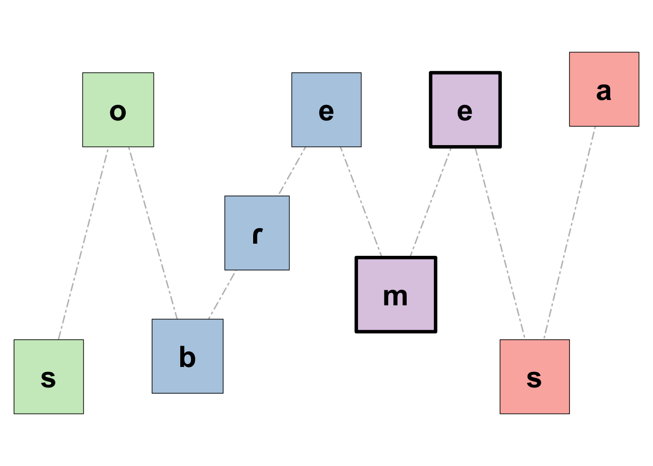
The function plotSon() creates a plot using ggplot2 to visualize the sonority profile of a given word, which must be phonemically transcribed. This is adapted from the Shiny App you can find here. If you want the figure to differentiate the syllables in the word of interest (syl = T), your input must also be syllabified (in that case, the stressed syllable will be highlighted with thicker borders). Finally, if you want to save your figure, simply add save_plot = T to the function. The function has a relatively flexible phonemic inventory. If a phoneme isn’t supported, the function will print it (and the figure won’t be generated). The sonority scale used here can be found in Parker (2011).
"combradol" |>
  ipa() |>
  plotSon(syl = F)

"sobremesa" |>
  ipa(lg = "sp") |>
  plotSon(syl = T)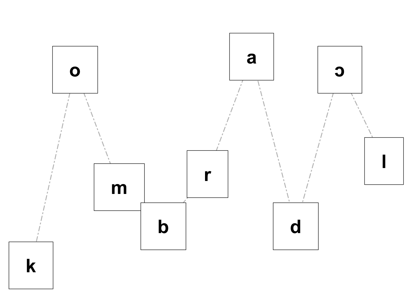
Bigram probabilities
The function biGram_pt() returns the log bigram probability for a possible word in Portuguese (word must be broadly transcribed). The string must use broad phonemic transcription, but no syllabification or stress. The reference used to calculate probabilities is the Portuguese Stress Lexicon.
biGram_pt("paklode")
#> [1] -43.11171
Two additional functions can be used to explore bigrams: nGramTbl() generates a tibble with phonotactic bigrams from a given text, and plotnGrams() creates a plot for inputs generated with nGramTbl(). Check ?plotnGrams() for more information.
Word generator for Portuguese
The function wug_pt() generates a hypothetical word in Portuguese. Note that this function is meant to be used to get you started with nonce words. You will most likely want to make adjustments based on phonotactic preferences. The function already takes care of some OCP effects and it also prohibits more than one onset cluster per word, since that’s relatively rare in Portuguese. Still, there will certainly be other sequences that sound less natural. The function is not too strict because you may have a wide range of variables in mind as you create novel words. Finally, if you wish to include palatalization, set palatalization = T—if you do that, biGram_pt() will de-palatalize words for its calculation, as it’s based on phonemic transcription.
set.seed(1)
wug_pt(profile = "LHL")
#> [1] "dra.ˈbur.me"
# Let's create a table with 5 nonce words
# and their bigram probabilities
set.seed(1)
tibble(word = character(5)) |>
mutate(word = wug_pt("LHL", n = 5),
bigram = word |>
biGram_pt())| word | bigram |
|---|---|
| dra.ˈbur.me | -118.61127 |
| ze.ˈfran.ka | -85.59775 |
| be.ˈʒan.tre | -84.75405 |
| ʒa.ˈgran.fe | -87.60279 |
| me.ˈxes.vro | -100.89858 |
Plotting vowels
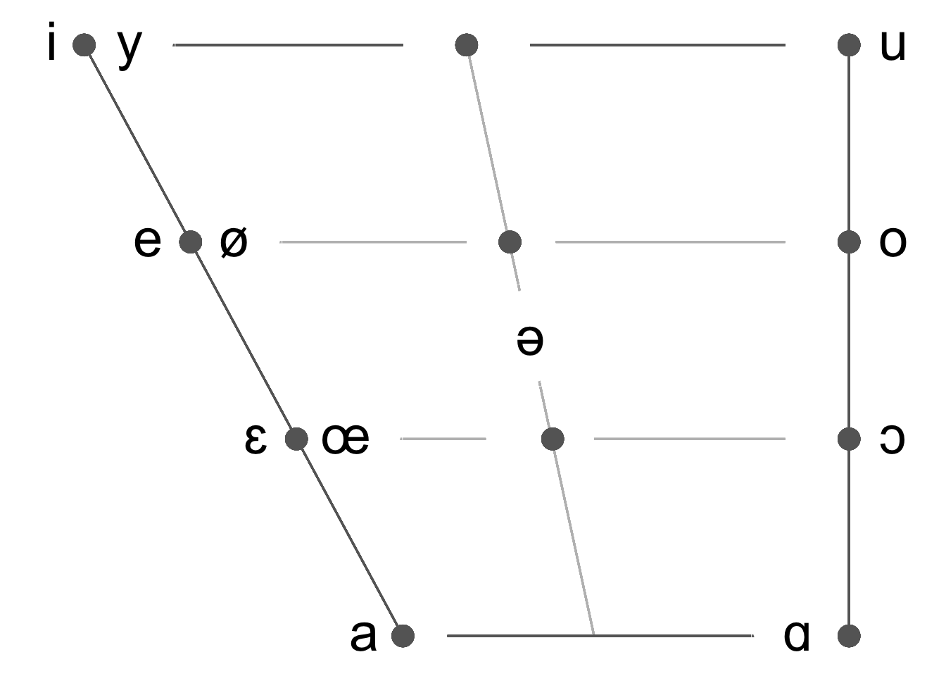
The function plotVowels() creates a vowel trapezoid using ggplot2. If tex = T, the function also saves a tex file with the LaTeX code to create the same trapezoid using the vowel package. Available languages: Arabic, French, English, Dutch, German, Hindi, Italian, Japanese, Korean, Mandarin, Portuguese, Spanish, Swahili, Russian, Talian, Thai, and Vietnamese. Only oral monophthongs are plotted. This function is also implemented as a Shiny App here.
plotVowels(lg = "Spanish", tex = F)
plotVowels(lg = "French", tex = F)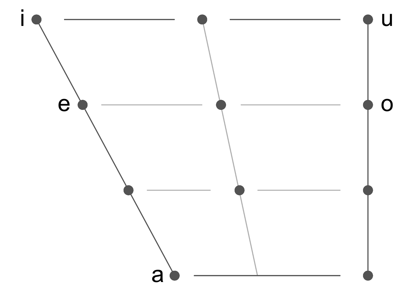
If you use Typst, this function has been superseded by phonokit (function #vowels()).
From IPA to TIPA or Typst
The function ipa2tipa() takes a phonemically transcribed sequence and returns its tipa equivalent, which can be handy if you use \(\LaTeX\). Alternatively, you can use ipa2typst(), which will output a string to be used with phonokit’s #ipa() function.
"Aqui estão algumas palavras" |>
  cleanText() |>
  ipa(narrow = T) |>
  ipa2tipa()
#> Done! Here's your tex code using TIPA:
#> \textipa{ / a."ki es."t\~{a}\~{w} aw."g\~{u}.mas pa."la.vRas / }
Working with ages in acquisition studies
It’s very common to use the format yy;mm for children’s ages in language acquisition studies. To make it easier to work with this format, two functions have been added to the package: monthsAge(), which returns an age in months given a yy;mm age, and meanAge(), which returns the average age of a vector using the same format (in both functions, you can specify the year-month separator). Here are a couple of examples:
monthsAge(age = "02;06")
#> [1] 30
monthsAge(age = "05:03", sep = ":")
#> [1] 63

meanAge(age = c("02;06", "03;04", NA))
#> [1] "2;11"
meanAge(age = c("05:03", "04:07"), sep = ":")
#> [1] "4:11"Acknowledgements and funding
Parts of this project have benefited from funding from the ENVOL program at Université Laval and from the Social Sciences and Humanities Research Council of Canada (SSHRC). Different undergraduate research assistants at Université Laval have worked on the Spanish and French grapheme-to-phoneme conversion functions: Nicolas C. Bustos, Emmy Dumont, and Linda Wong. Matéo Levesque implemented comprehensive regular expressions for French transcription. French lookup data are derived from Lexique 4 (New et al., 2026), distributed through OpenLexicon under CC BY-SA 4.0. Italian and Spanish lookup data are derived from the English Wiktionary via Wiktextract, as distributed by kaikki.org; Wiktionary content is available under CC BY-SA. English lookup data are derived from the CMU Pronouncing Dictionary.
Citing the package
citation("Fonology")
#> To cite Fonology in publications, use:
#>
#>   Garcia, Guilherme D. (2026). Fonology: Phonological Analysis in R. R
#>   package version 1.2.0 (first published 2023, latest 2026). Available
#>   at https://gdgarcia.ca/fonology
#>
#> A BibTeX entry for LaTeX users is
#>
#>   @Manual{,
#>     title = {Fonology: Phonological Analysis in {R}},
#>     author = {Guilherme D. Garcia},
#>     note = {R package version 1.2.0 (first published 2023, latest 2026)},
#>     year = {2026},
#>     url = {https://gdgarcia.ca/fonology},
#>   }
Copyright © Guilherme Duarte Garcia
References
Clements, G. N. (1990). The role of the sonority cycle in core syllabification. In J. Kingston & M. Beckman (Eds.), Papers in Laboratory phonology 1: Between the grammar and physics of speech (pp. 283–333). Cambridge University Press.
Garcia, G. D. (2026). Fonology: Phonological analysis in R. https://doi.org/10.5281/zenodo.19958335
Goldwater, S., & Johnson, M. (2003). Learning OT constraint rankings using a Maximum Entropy model. Proceedings of the Stockholm Workshop on Variation Within Optimality Theory, 111–120.
Hayes, B., & Wilson, C. (2008). A Maximum Entropy model of phonotactics and phonotactic learning. Linguistic Inquiry, 39(3), 379–440. https://doi.org/10.1162/ling.2008.39.3.379
Mayer, C., Tan, A., & Zuraw, K. R. (2024). Introducing
maxent.ot: An R package for Maximum Entropy constraint grammars. Phonological Data and Analysis, 6(4), 1–44. https://doi.org/10.3765/pda.v6art4.88
New, B., Pallier, C., Schalchli, G., Bourgin, J., & Gimenes, M. (2026). Lexique 4: A major upgrade of the Lexique French lexical database. Behavior Research Methods. http://www.lexique.org/databases/Lexique400/Lexique400.pdf
Parker, S. (2011). Sonority. In M. van Oostendorp, C. J. Ewen, E. Hume, & K. Rice (Eds.), The Blackwell companion to phonology (pp. 1160–1184). Wiley Online Library. https://doi.org/10.1002/9781444335262.wbctp0049
Wijffels, J. (2023). Udpipe: Tokenization, parts of speech tagging, lemmatization and dependency parsing with the ’UDPipe’ ’NLP’ toolkit. https://CRAN.R-project.org/package=udpipe
Wilson, C. (2006). Learning phonology with substantive bias: An experimental and computational study of velar palatalization. Cognitive Science, 30(5), 945–982. https://doi.org/10.1207/s15516709cog0000_89